Download
1 / 56
610 likes | 842 Vues
Introduction to complex networks Part II: Models. NetSci 2010 Boston, May 10 2010. Ginestra Bianconi Physics Department,Northeastern University, Boston,USA. Random graphs. G(N,L) ensemble Graphs with exactly N nodes and L links. G(N,p) ensemble Graphs with N nodes

E N D
Introduction to complex networksPart II: Models NetSci 2010 Boston, May 10 2010 Ginestra Bianconi Physics Department,Northeastern University, Boston,USA
Random graphs G(N,L) ensemble Graphs with exactly N nodes and L links G(N,p) ensemble Graphs with N nodes Each pair of nodes linked with probability p Binomial Poisson distribution distribution
Random graphs G(N,L) ensemble Graphs with exactly N nodes and L links Poisson distribution Small clustering coefficient Small average distance
Regular lattices • d dimensions • Large average distance • Significant local interactions
Universalities:Small world i # of links between 1,2,…ki neighbors Ci = ki(ki-1)/2 Ki Networks are clustered (large average Ci,i.e.C) but have a small characteristic path length (small L). Watts and Strogatz (1999)
Watts and Strogatz small world model Watts & Strogatz (1998) Variations and characterizations Amaral & Barthélemy(1999) Newman & Watts, (1999) Barrat & Weigt, (2000) There is a wide range of values of p in which high clustering coefficient coexist with small average distance
Small world and efficiency • Small worlds are both locally and globally efficient • Boston T is only globally efficient Latora & Marchiori 2001, 2002
Degree distribution of the small world model The degree distribution of the small-world model is homogeneous Barrat and Weigt 2000
Universalities:Scale-free degree distribution Actor networks WWW Internet k k Faloutsos et al. 1999 Barabasi-Albert 1999
Scale-free networks • Technological networks: • Internet, World-Wide Web • Biological networks : • Metabolic networks, • protein-interaction networks, • transcription networks • Transportation networks: • Airport networks • Social networks: • Collaboration networks • citation networks • Economical networks: • Networks of shareholders in the financial market • World Trade Web
Why this universality? • Growing networks: • Preferential attachment Barabasi & Albert 1999, Dorogovtsev Mendes 2000,Bianconi & Barabasi 2001, etc. • Static networks: • Hidden variables mechanism Chung & Lu 2002, Caldarelli et al. 2002, Park & Newman 2003
Motivation for BA model 1) The network grow Networks continuously expand by the addition of new nodes Ex. WWW : addition of new documents Citation : publication of new papers 2) The attachment is not uniform (preferential attachment). A node is linked with higher probability to a node that already has a large number of links. Ex: WWW : new documents link to well known sites (CNN, YAHOO, NewYork Times, etc) Citation : well cited papers are more likely to be cited again
BA model P(k) ~k-3 (1)GROWTH: At every timestep we add a new node with m edges (connected to the nodes already present in the system). (2)PREFERENTIAL ATTACHMENT :The probability Π that a new node will be connected to node i depends on the connectivity ki of that node Barabási et al. Science (1999)
Result of the BA scale-free model • The connectivity of each node increases in time as a power-law with exponent 1/2: • The probability that a node has k links follow a power-law with exponent =3:
Initial attractiveness A preferential attachment with initial attractiveness A yields The initial attractiveness can change the value of the power-law exponent Dorogovtsev et al. 2000
Non-linear preferential attachment • <1 Absence of power-law degree distribution • =1 Power-law degree distribution • >1 Gelation phenomena The oldest node acquire most of the links First-mover-advantage Krapivski et al 2000
Gene duplication model • Duplication of a gene adds a node. • New proteins will be preferentially connected to high connectivity. Effective preferential attachment A. Vazquez et al. (2003).
Other variations Scale-free networks with high-clustering coefficient Dorogovtsev et al. 2001 Eguiluz & Klemm 2002 Aging of the nodes Dorogovstev & Medes 2000 Pseudofractal scale-free network Dorogovtsev et al 2002
Features of the nodes In complex networks nodes are generally heterogeneous and they are characterized by specific features • Social networks: age, gender, type of jobs, drinking and smoking habits, • Internet: position of routers in geographical space, … • Ecological networks: Trophic levels, metabolic rate, philogenetic distance • Protein interaction networks: localization of the protein inside the cell, protein concentration
Fitness the nodes Not all the nodes are the same! Let assign to each node an energy of a node In the limit =0 all the nodes have same fitness 6 1 3 2 5 4
The fitness model • Growth: • At each time a new node and m links are added to the network. • To each node i we assign a energy i from a p() distribution • Generalized preferential attachment: • Each node connects to the rest of the network by m links attached preferentially to well connected, low energy nodes. 6 1 3 2 5 4
Results of the model • Power-law degree distribution • Fit-get-rich mechanism
Fit-get rich mechanism The nodes with higher fitness increases the connectivity faster satisfies the condition
Mapping to a Bose gas 6 1 We can map the fitness model to a Bose gas with • density of states p( ); • specific volume v=1; • temperature T=1/. In this mapping, • each node of energy corresponds to an energy level of the Bose gas • while each link pointing to a node of energy ,corresponds to an occupation of that energy level. 3 2 5 4 Network Energy diagram G. Bianconi, A.-L. Barabási 2001
Bose-Einstein condensation in trees scale-free networks • In the network there is a critical temperature Tc such that • for T>Tc the network is in the • fit-get-rich phase • for T<Tc the network is in the • winner-takes-all • or Bose-condensatephase
Correlations in the Internetand the fitness model • knn (k) mean value of the connectivity of neighbors sites of a node with connectivity k • C(k) average clustering coefficient of nodes with connectivity k. Vazquez et al. 2002
Growing weighted models With new nodes arriving at each time Yook & Barabasi 2001 Barrat et al. 2004 With weight-degree correlations And possible condensation of the links G. Bianconi 2005
Growing Cayley-tree 7 • Each node is either at the interface ni=1 or in the bulk ni=0 • At each time step a node at the interface is attached to m new nodes with energies from a p( ) distribution. • High energy nodes at the interface are more likely to grow. • The probability that a node i grows is given by • G. Bianconi 2002 5 6 9 4 8 3 2 1 Nodes at the interface
Mapping to a Fermi gas The growing Cayley tree network can be mapped into a Fermi gas • with density of states p(); • temperature T=1/; • specific volume v=1-1/m. • In the mapping the nodescorresponds to the energy levels • the nodes at the interface to the occupied energy levels 7 5 6 9 4 8 3 2 Network Energy diagram 1
Why this universality? • Growing networks: • Preferential attachment Barabasi & Albert 1999, Dorogovtsev Mendes 2000, Bianconi & Barabasi 2001, etc. • Static networks: • Hidden variables mechanism Chung & Lu 2002, Caldarelli et al. 2002, Park & Newman 2003
Molloy Reed configuration model Networks with given degree distribution Assign to each node a degree from the given degree distribution Check that the sum of stubs is even Link the stubs randomly If tadpoles or double links are generated repeat the construction Molloy & Reed 1995
Caldarelli et al. hidden variable model • Every nodes is associated with an hidden variable xi • The each pair of nodes are linked with probability Caldarelli et al. 2002 Soderberg 2002 Boguna & Pastor-Satorras 2003
Park & Newman Hidden variables model J. Park and M. E. J. Newman (2004). The system is defined through an Hamiltonian pij is the probability of a link • The “hidden variables” i are quenched and distributed through the nodes with probability (). • There is a one-to-one correspondence between and the average connectivity of a node
Random graphs G(N,p) ensemble Graphs with N nodes Each pair of nodes linked with probability p G(N,L) ensemble Graphs with exactly N nodes and L links Binomial Poisson distribution distribution
Statistical mechanics and random graphs Statistical mechanics Random graphs Microcanonical Configurations G(N,L) Graphs Ensemble with fixed energyE Ensemble with fixed # of links L Canonical Configurations G(N,p) Graphs Ensemble with fixed average Ensemble with fixed average energy <E> #of links <L>
Gibbs entropy and entropy of the G(N,L) random graph Statistical mechanics Microcanonical ensemble Random graphs G(N,L) ensemble Entropy per node of the G(N,L) ensemble Gibbs Entropy Total number of microscopic configurations with energy E Total number of graphs in the G(N,L) ensembles
Shannon entropy and entropy of the G(N,p) random graph Statistical mechanics Canonical ensemble Random graphs G(N,p) ensemble Entropy per node of the G(N,p) ensemble Shannon Entropy Typical number of microscopic configurations with temperature b Total number of typical graphs the G(N,p) ensembles
Complexity of a real network Hypothesis: Real networks are single instances of an ensemble of possible networks which would equally well perform the function of the existing network The “complexity” of a real network is a decreasing function of the entropy of this ensemble G. Bianconi EPL (2008)
Citrate cycle:highly preserved Homo Sapiens Escherichia coli
The complexity of networks is indicated by their organization at different levels • Average degree of a network • Degree sequence • Degree correlations • Loop structure • Clique structure • Community structure • Motifs
Relevance of a network characteristics How many networks have the same: Entropy of network ensembles with given features Degree sequence Added features Degree correlations The relevance of an additional feature is quantified by the entropy drop Communities
Networks with given degree sequence Microcanonical ensemble Canonical ensemble Ensemble of network with exactly M linksEnsemble of networks with average number of links M Molloy-Reed Hidden variables
Shannon Entropy of canonical ensembles We can obtain canonical ensembles by maximizing this entropy conditional to given constraints
Link probabilities Constraints Link probability • Total number of links L=cN • Degree sequence {ki} • Degree sequence {ki} and number of links in within and in between communities {qi} • In spatial networks, degree sequence {ki} and number of links at distance d Anand & Bianconi PRE 2009
Partition function randomized microcanonical network ensembles Statistical mechanics on the adjacency matrix of the network hij auxiliary fields
The entropy of the randomized ensembles Gibbs Entropy per node of a randomized network ensemble Probability of a link.
The link probabilitiesin microcanonical and canonical ensembles are the same -Example Microcanonical ensembleCanonical ensemble Regular networksPoisson networks but Anand & Bianconi 2009
Two examples of given degree sequence Non-zero entropy Zero entropy k=2 k=2 k=3 k=1 k=2
The entropy of random scale-free networks The entropy decreases as decrease toward 2 quantifying a higher order in networks with fatter tails Bianconi 2008
Change and Necessity: Randomness is not all Selection or non-equilibrium processes have to play a role in the evolution of highly organized networks