Download
1 / 14
140 likes | 233 Vues
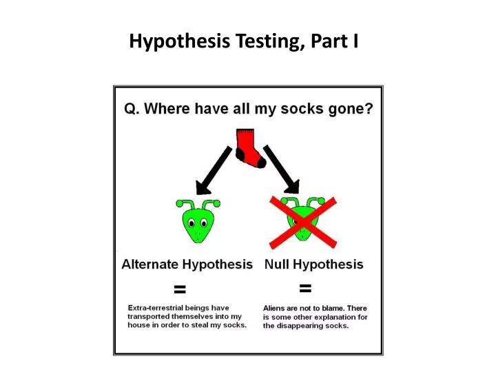
Hypothesis Testing, Part I. Learning Objectives. By the end of this lecture, you should be able to: Describe what is meant by null hypothesis and alternative hypothesis. Describe the general principles guiding what to call H 0 and H a .

E N D
Learning Objectives By the end of this lecture, you should be able to: • Describe what is meant by null hypothesis and alternative hypothesis. • Describe the general principles guiding what to call H0 and Ha. • Describe what is meant by ‘reject the null hypothesis’ and ‘fail to reject the null hypothesis’. • Give examples of setting up a hypothesis test between two groups. • Explain, using an example(s), how the size of the difference between the groups, and the size of the sample play a key role in determining whether there is a difference between the two groups being examined.
Circular Learning • There are a few tricky terms and concepts in the subject of hypothesis testing and statistical significance. • A good way to go about it is to go through the topic 2-3 times. Each time you return to it, certain aspects should become increasingly clear. • No matter how slow you take it, don’t expect everything to make sense on the first go. By all means, take your time, and stop and think about the concepts as they are discussed. • However, once you’ve seen various examples and tried some on your own, you’ll find many of the topics in these notes are much more clear upon a second, third (etc) look.
Overview Example This example forms the entire basis for this discussion. Statistical significance is one of the most widely misunderstood concepts in statistics as it is applied to the real world. Review this example every little while as you study the chapter. It will help the ‘big picture’ emerge. Researchers at a hospital want to know if a new drug is more effective than an older version of the drug. Twenty patients receive the new drug, and 20 receive the old medication. 11 (55%) of those taking the new drug show improvement versus only 8 (40%) of the patients on the older drug. Our unaided judgement would suggest that the new drug is better. However, various calculations tell us that a difference between the two groups that is this large (15%) or even larger would occur about 1 in 5 times purely by chance. That is, even if there was NO difference (e.g. suppose both groups showed 60% improvement), 1/5 times we’d see a difference this size (15%) or larger. In significance testing, a 1/5 probability is not considered to be small. Ultimately, rather than make any major, expensive changes in medication at the hospital, it is better to conclude that the observed difference between those two groups was purely due to chance rather than to any real difference between the two medications. • Yes, the likelihood that this result was due to chance (a fluke) is only 1/5 (20%). But in significance testing, we typically consider this value as too high to ignore. In addition to understanding the big picture, you will also learn how to determine the probability that some result was due to chance (the “1/5”) we came up with above.
Example You are in charge of quality control in your food company. You randomly sample four packs of cherry tomatoes, that you company labels 1/2 lb. (227 g). The average weight of your sample of four boxes is 222 g. Oh NO!!!! Are we going to get sued for misleading our customers? Do we have to go back and recalibrate all of the machines in our factories? Probably not… Any thoughts on why we shouldn’t panic based on this test? Answer: In this example, our sample size is quite small. Ultimately, we will see that we can confidently state that the results of our experiment were “not statistically significant”.
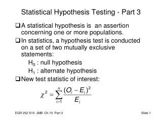
Terms In statistics, a hypothesis is an assumption or theory about the characteristics of a variable(s) in a population. A test of statistical significance tests a specific hypothesis (theory) using data obtained from a sample. In order to decide if a result is statistically significant, we must apply a hypothesis test.
Terminology The null hypothesis is a (very) specific statement about some parameter of the population. It is labeled H0 . The alternative hypothesis is a statement about the same parameter of the population that is exclusive of the null hypothesis. It is labeled Ha. Weight of cherry tomato packs: H0 : µ = 227 g (µis the average weight of the population of packs) Ha : µ ≠ 227 g (µ is either larger or smaller than 227g)
Deciding on H0 v.s. Ha It is up to us to decide what to call H0 and what to call Ha. Typically though, we call what WE are trying to prove Ha, and we call the status-quo, or any opposing claim, H0. That being said, it’s still up to you to decide what to label as H0 and what to label as Ha. Example: A cigarette manufacturer claims that its nicotine levels are no higher than 1.4. A personal injury attorney has hired you to take a sample and prove that they are lying. Set H0 to be the evidence you are trying to DIS-prove. Ha is what you are trying to prove. • Your hypothesis, is that the nicotine is >1.4 • Ha: nicotine > 1.4 • Because you are hoping to prove that the company is lying, you should set up the null hypothesis as the default value: • Ho : nicotine <= 1.4
Examples – Identify H0 and Ha Deciding exactly what to call H0 and what to call Ha is not set in stone. But generally, we take the hypothesis we are trying to “prove” and call it Ha. Hypothesis: The mean weight of people in Illinois is higher than the mean weight of people in California. • Ha: mean wt in IL > mean weight in CA • H0: mean wt in IL <= mean weight CA Hypothesis: A tobacco company claims that their nicotine levels are no greater than 1.4. We believe they are not being entirely truthful, and suspect that the average amount of nicotine in a pack of cigarettes is, in fact, greater than 1.4. • Ha: nicotine > 1.4 • H0: nicotine <= 1.4 Hypothesis: You are worried that your company’s machines are mis-calibrated, and that the the average weight of a package of cherry tomatoes is no longer 227 grams. • Ha: mean weight ≠ 227g • H0: mean weight = 227g
“Rejecting the Null Hypothesis” • Recall that in a previous example, the null hypothesis H0 stated that: H0: Nicotine levels are less than or equal to 1.4 • If your sample shows that the nicotine levels are greater than 1.4, you “reject the null hypothesis”. • Typically, experiments are trying to prove something unusual. That is, typically we are trying to reject the null hypothesis. • If your sample does NOT fail to prove this result, then you “fail to reject the null hypothesis”. • Admittedly, there are lots of negative here: “Fail” to “reject” the “null” hypothesis! But you do have to be comfortable with them. It just takes a little getting used to. This comes with ____________ ???? • And do review it! Here is an entirely non-subtle hint from your prof: “I promise to incldue questions on this terminology on both quizzes and exams!“ Clear enough?
Significance testing begins with a comparison Here are some types of comparisons that are commonly encountered: • The value from a sample v.s. the value from a previously accepted value • Your company has been packaging tomatoes and labeling the average weight as being 227 grams. You want to confirm that the current weight is not less than this value. • You might compare: H0: mean weight = 227 with Ha: mean weight ≠ 227 • The value from a sample v.s. a value that has been “claimed” • A cigarette company claims that their nicotine levels are no more than 1.4. • You might compare the H0: nicotine <= 1.4 with Ha: nicotine > 1.4 • The value of a sample taken from one population v.s. the value from a sample taken from another population • We want to see if people in Illinois are more fit, and therefore weigh less than people who live in California. • You might compare: H0: mean weight IL > mean weight CA v.s. Ha: mean weight Il <= mean weight CA.
Think about it intuitively for a moment… • Very generally speaking, if the difference between the the two groups we are comparing is extremely small, we might intuitively appreciate that is may well be due to chance. • Mean weight 1000 people in Illinois = 156.5 pounds. • Mean weight 1000 people in California = 156.3 pounds. • We recognize that different samples will give different values (i.e. sampling variability), and that therefore, it is entirely possible that this very small difference may be due purely to chance (sampling variability.) • Similarly, If the difference between the the two groups we are comparing is extremely large, we are much more likely to intuit that this difference is not very likely to be due to chance. • Mean weight 1000 people in Illinois = 156.5 pounds. • Mean weight 1000 people in California = 129.2 pounds. • Even though different samples will give different values, the probability of finding such a large difference purely by chance is quite small. That is, there very likely IS a real differnce between the two groups. Therefore, in this case, it is quite UN-likely that the difference between the two groups is due to chance. A hypothesis test is a calculation comes up with a probability value of the likelihood that the difference in size between the two groups is due to chance.
Size of the Difference & Size of the Sample The purpose of a significance test is to determine whether or not the difference between the two means that we are comparing could be due to sampling variability (i.e. chance). • Suppose one group of people (e.g. people in Illinois) has an average weight of 156 pounds and a different group (e.g. people in California) has an average weight of 157 pounds So: Illinois mean = 156, California mean = 157. Can we confidently report that people from Illinois weigh less than people from California? • NO! The reason is that all samples vary. In other words, it is entirely possible that if you took another sample from Illinois, you might end up with, say, 158 pounds. Would you then promptly change your mind and now report that Illinoisans weight more than Californians? Again, I hope you agree that the answer is NO. • Now suppose your sample from Illinois has a mean weight of 180 pounds and the sample from CA has a mean weight of 140 pounds. In this case, you are somewhat more safe in assuming that there is a genuine difference in weights between the groups. • However, there is still a limitation – do you see it??? • What if I told you that the group from Illinois had only two people in the sample?! In this case, we would not place much trust in the value obtained for the mean. • KEY POINT: In order to determine whether or not there truly is a difference between Group 1 and Group 2, we are interested in two key items: • The size of the difference between the two groups. (e.g. 1 pounds g v.s. 40 pounds) • The size of the sample used in each of the groups (e.g. 500 people v.s. 2 people) • When we finally get to actual calculations of a hypothesis test, you will see that both of these factors (size of the difference and size of the sample) come into play.
Example of key factors • We wish to determine whether the weight of a package of chery tomatoes as determined from our sample is truly different from the advertised weight (H0). • We weigh four packages and find the average weight = 222 g • Weight advertised = 227 g • In this case, the difference is only 5 grams. Perhaps we are misleading our customers. However, note that our sample was only 4 packages. Could we BY CHANCE happened to have chosen a few packages that were smaller than usual? The answer depends on two key factors: The size of the difference between the two groups: In this case, the difference between the groups was only 5 grams which seems fairly small. It is plausible that given our small sample size, we may BY CHANCE have gotten a few slightly smaller than average packages. • Suppose that our sample came out to 226.9 grams (i.e. the difference was 0.1 grams). Do you agree that it seems very likely that there is no difference between the sample and H0? Isn’t is entirely possible that if we took another sample, we might just as easily end up with a mean weight greater than 227 (e.g. 227.3 g)? • Suppose our average weight from the sample was 160 grams (i.e. the difference was 67 grams). In this case, even with a small sample size (only 4 packages), a difference so large (67g) is unlikely to be due to sampling variability. The size of the sample (‘n’):In this case, we only used 4 packages. I am not sure that we can accept that a 5 g difference is real. There is a very reasonable chance that it is due to sampling variability. If, however, we had sampled, say, 2000 packages and found a 5g difference, we can also be fairly sure that a this difference was not due to sampling variability.