Relationships Regression

1. RelationshipsRegression BPS chapter 5 © 2006 W.H. Freeman and Company

2. Objectives (BPS chapter 5) Regression • Regression lines • The least-squares regression line • Using technology • Facts about least-squares regression • Residuals • Influential observations • Cautions about correlation and regression • Association does not imply causation

3. Correlation tells us about strength (scatter) and direction of the linear relationship between two quantitative variables. In addition, we would like to have a numerical description of how both variables vary together. For instance, is one variable increasing faster than the other one? And we would like to make predictions based on that numerical description. But which line best describes our data?

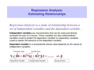
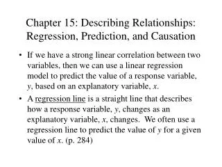
4. A regression line (page 115) A regression line is a straight line that describes how a response variable y changes as an explanatory variable x changes. We often use a regression line to predict the value of y for a given value of x.

5. The distances between the data points and the line are called the residuals (more on this later)… The regression line (page 119) The least-squares regression line is the unique line such that the sum of the squaredvertical (y) distances between the data points and the line is the smallest possible.

6. Facts about least-squares regression • The distinction between explanatory and response variables is essential in regression. (Don’t mix up x and y) • There is a close connection between correlation and the slope of the least-squares line. (r is used in the formula for the slope) • The least-squares regression line always passes through the point • The correlation r describes the strength of a straight-line relationship. The square of the correlation, r2, is the fraction of the variation in the values of y that is explained by the least-squares regression of y on x. (This will make more sense shortly) Centroid!

7. Is this the y-intercept? Line Basics and Properties We will write the least-squares regression using the equation: is the predicted y value (y hat) b is the slope (rise over run) a is the y-intercept (when x=0) "a" is in units of y "b" is in (units of y)/(units of x)

8. Sample Statistics and the Least Square Line The slope b and y-intercept a of the least squares line are closely related to the sample means and standard deviations of the x and y data: The slope of the line, b, is the standard deviation of y divided by the standard deviation of x , and weighted by the correlation r r is the correlation sy is the “statistical change” in y sx is the “statistical change” in x Once we know b, the slope, we can calculate a, the y-intercept: where x and y are the sample means of the x and y variables

9. Find the LS Regression Line By Hand: Which variable is the explanatory variable (i.e. x)? Which is the response variable (i.e. y)? Given that the correlation between these two variables is r = -0.9442, can you use the previous formulae to find the equation of the least-squares regression line?

10. Now Let’s Use Our Calculators: • Let’s Get the Equation of the least-squares regression line for our Absence and Final Grade Data (It should still be in L1 and L2) • Make sure you have turned your Diagnostics On: 2nd Catalog, scroll down to DiagnosticOn and press Enter (you do not have to repeat this step everytime!) • Stat|Calc|LinReg(a+bx) L1,L2 gives: y=a+bx where: a=102.49, b=-3.622, r^2=0.8915 and r=-0.9442 • So the equation of the least-squares regression line is: Predicted Final Grade = 102.49 – 3.622*(Number of Absences)

11. BEWARE !!! Not all calculators and software use the same convention: Some use instead: Make sure you know what YOUR calculator gives you for a and b before you answer homework or exam questions.

12. Let’s plot the regression line we just found:

13. Making predictions: Interpolation The equation of the least-squares regression allows you to predict y for any xwithin the range studied. This is called interpolating. Based on our data, what final grade would we expect if a student had 10 absences? x = 10 y = -3.6219 (10) + 102.49 = 66.271 ^ This is our predicted y-value!

14. (in 1000’s) There is a positive linear relationship between the number of powerboats registered and the number of manatee deaths. The least-squares regression line has for equation: Thus, if we were to limit the number of powerboat registrations to 500,000, what could we expect for the number of manatee deaths? Roughly 21 manatees.

15. Data from the Hubble telescope about galaxies moving away from Earth: These two lines are the two regression lines calculated either correctly (x = distance, y = velocity, solid line) or incorrectly (x = velocity, y = distance, dotted line). The distinction between explanatory and response variables is crucial in regression. If you exchange y for x in calculating the regression line, you will get the wrong line. Regression examines the distance of all points from the line in the y direction only.

16. Correlation and regression The correlation is a measure of spread (scatter) in both the x and y directions in the linear relationship. In regression we examine the variation in the response variable (y) given change in the explanatory variable (x).

17. Coefficient of determination, r2 r2 represents the fraction of the variance in y(vertical scatter from the regression line) that can be explained by changes in x. What do we mean by that??? r2, the coefficient of determination, is the square of the correlation coefficient.

18. r = 0.87 r2 = 0.76 Changes in x explain 0% of the variations in y. The value(s) y takes is (are) entirely independent of what value x takes. r = 0 r2 = 0 Here the change in x only explains 76% of the change in y. The rest of the change in y (the vertical scatter, shown as red arrows) must be explained by something other than x. r = −1 r2 = 1 Changes in x explain 100% of the variations in y. y can be entirely predicted for any given value of x.

19. We changed the number of beers to the number of beers/weight of a person in pounds. r =0.9 r2 =0.81 There is quite some variation in BAC for the same number of beers drunk. A person’s blood volume is a factor in the equation that was overlooked here. r =0.7 r2 =0.49 • In the first plot, number of beers only explains 49% of the variation in blood alcohol content. • But number of beers/weight explains 81% of the variation in blood alcohol content. • Additional factors contribute to variations in BAC among individuals (like maybe some genetic ability to process alcohol).

20. Grade performanceThere is a positive association between SAT scores and grades. If SAT score explains 16% of the variation in grades for a certain class, what is the correlation between percent of SAT score and grade?1. SAT score and grades are positively correlated. So r will be positive too. 2. r2 = 0.16, so r = +√0.16 = + 0.4 A weak correlation. 3. For our example Absences example, what percent of the variation in grades was explained by the number of absences? 89.15%

21. Points above the line have a positive residual. Points below the line have a negative residual. Residuals The distances from each point to the least-squares regression line give us potentially useful information about the contribution of individual data points to the overall pattern of scatter. These distances are called “residuals.” The sum of theseresiduals is always 0. ^ Predicted y Observed y

22. Residual plots Residuals are the distances between y-observed and y-predicted. We plot them in a residual plot. If residuals are scattered randomly around 0, chances are your data fit a linear model, were normally distributed, and you didn’t have outliers.

23. The x-axis in a residual plot is the same as on the scatterplot. • The line on both plots is the regression line. Only the y-axis is different.

24. Residuals are randomly scattered—good! A curved pattern—means the relationship you are looking at is not linear. A change in variability across plot is a warning sign. You need to find out why it is and remember that predictions made in areas of larger variability will not be as good.

25. Child 19 = outlier in y direction Child 19 is an outlier of the relationship. Child 18 is only an outlier in the x direction and thus might be an influential point. Child 18 = outlier in x direction Outliers and influential points Outlier: An observation that lies outside the overall pattern of observations. “Influential individual”: An observation that markedly changes the regression if removed. This is often an outlier on the x-axis.

26. Outlier in y-direction Influential All data Without child 18 Without child 19 Are these points influential?

27. Correlation/regression using averages Many regression or correlation studies use average data. While this is appropriate, you should know that correlations based on averages are usually quite higher than when made on the raw data. The correlation is a measure of spread (scatter) in a linear relationship. Using averages greatly reduces the scatter. Therefore, r and r2 are typically greatly increased when averages are used.

28. Boys These histograms illustrate that each mean represents a distribution of boys of a particular age. Boys Each dot represents an average. The variation among boys per age class is not shown. Should parents be worried if their son does not match the point for his age? If the raw values were used in the correlation instead of the mean, there would be a lot of spread in the y-direction ,and thus, the correlation would be smaller.

29. That’s why typically growth charts show a range of values (here from 5th to 95th percentiles). This is a more comprehensive way of displaying the same information.

30. Caution with regression • Do not use a regression on inappropriate data. • Pattern in the residuals • Presence of large outliers Use residual plots for help. • Clumped data falsely appearing linear • Recognize when the correlation/regression is performed on averages. • A relationship, however strong, does not itself imply causation. • Beware of lurking variables. • Avoid extrapolating (going beyond interpolation).

31. Lurking variables A lurking variable is a variable not included in the study design that does have an effect on the variables studied. Lurking variables can falsely suggest a relationship. What are potential lurking variables in these examples? How could you answer if you didn’t know anything about the topic? • There is a strong positive association between the amount of artificial sweetener a person uses and that person’s weight. • So artifical sweeteners cause people to gain weight? • Most of the states with the lowest murder rates do not have a death penalty; most of the states with the highest murder rates do.1 • So the death penalty actually causes an increase in murder rates? • Murder rates have increased in the UK and Australia since stricter gun control laws were enacted in the late 1990’s. • So gun control laws actually cause higher murder rates? 1 http://www.deathpenaltyinfo.org/article.php?did=169

32. Association and causation Association, however strong, does NOT imply causation. Only careful experimentation can show causation. Not all examples are so obvious…

33. Note how much smaller the variation is. An individual’s weight was indeed influencing our response variable “blood alcohol content.” Lurking variables can also weaken associations… There is quite some variation in BAC for the same number of beers drunk. A person’s blood volume is a factor in the equation that we have overlooked. Now we change the number of beers to the number of beers/weight of a person in pounds.

34. Vocabulary: lurking vs. confounding LURKING VARIABLE • A lurking variable is a variable that is not among the explanatory or response variables in a study and yet may influence the interpretation of relationships among those variables. CONFOUNDING • Two variables are confounded when their effects on a response variable cannot be distinguished from each other. The confounded variables may be either explanatory variables or lurking variables. But you often see them used interchangeably…

35. The following all indicate that there is, in fact, a causal relationship between smoking and cancer: • The association is strong. • The association is consistent. • Higher doses are associated with stronger responses. • The alleged cause precedes the effect. • The alleged cause is plausible. Association and causation It appears that lung cancer is associated with smoking. How do we know that both of these variables are not being affected by an unobserved third (lurking) variable? For instance, what if there is a genetic predisposition that causes people to both get lung cancer and become addicted to smoking, but the smoking itself doesn’t cause lung cancer?

36. !!! !!! Extrapolation Extrapolation is the use of a regression line for predictions outside the range of x values used to obtain the line. This can be a very dangerous thing to do, as seen here. Height in Inches Height in Inches

37. Bacterial growth rate changes over time in closed cultures: If you only observed bacterial growth in test tubes during a small subset of the time shown here, you could get almost any regression line imaginable. Extrapolation can be a big mistake

38. The y-intercept Sometimes the y-intercept is not biologically possible. Here we have negative blood alcohol content, which makes no sense… y-intercept shows negative blood alcohol But the negative value is appropriate for the equation of the regression line. There is a lot of scatter in the data and the line is just an estimate.

39. Always plot your data! The correlations all give r ≈ 0.816, and the regression lines are all approximately = 3 + 0.5x. For all four sets, we would predict = 8 when x = 10.

40. Always plot your data! However, making the scatterplots shows us that the correlation/ regression analysis is not appropriate for all data sets. Moderate linear association; regression OK. One point deviates from the (highly linear) pattern of the other points; it requires examination before a regression can be done. Just one very influential point and a series of other points all with the same x value; a redesign is due here… Obvious nonlinear relationship; regression inappropriate.