Lecture 10

1. Lecture 10 Queueing Theory

2. Introduction There are a few basic elements common to almost all queueing theory application. Customers arrive, they wait for service in one or more queues, they receive some service and they leave. The relationship between arrivals, number of customers in a system and time in the system is given in the simple expression, (1) where, L = the average number of customers in the system      = the average arrival rate of entering customers W = the average amount of time that a customer spends in the system Excerpts from: Introduction to Probability Models, S. M. Ross, Academic Press

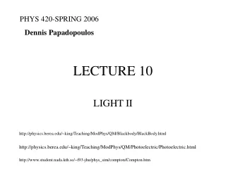
3. the "system" la server queue . . . arriving customers m served customer leaves system L Variations on a Theme Variations include systems with an infinite queue, systems with a finite queue, and systems with no queue. We will first study single-server, single-queue systems with infinite queue capacity. We will assume that the arrival time of the next customer is random with a measurable average arrival rate. This is called a Poisson (also Markovian or memoryless) process with an arrival rate of      . We will also assume an exponentially distributed service rate with mean,µ.

4. la . . . m L State of the System We will define the state of a system by the number of customers in the system. So that a system in state S0 is empty, a system in state S1 contains a single customer and a system in state Sncontains n customers. When customers first begin arriving, the system begins to fill with customers. If the arrival rate exceeds the service rate µ, the number of customers in the system will continue to grow without limit. (not interesting) On the other hand, if the service rate is greater than or equal to the arrival rate, the number of customers in the system will begin to level off or to achieve a steady state. We are interested in knowing the average number of customers in the system and the average time a customer must spend in the system when it is in its steady state.

5. The Principle of Balance Let us assume that we know the arrival and service rates for a single-server system in the steady state. We want to derive the quantities L and W in terms of and µ. We will use the principle of balance to help us in this derivation: For any system in the steady state, the rate at which it enters a state Sn equals the rate at which it leaves that state. The principle of balance can also be described in terms of the probability or proportion of time a system is in a particular state. If all proportions are constant, which they must be in the steady state, the rate of arrival of the system into a state must equal the rate of departure of the system from that state. First we look at a system entering and leaving the state S0. Our first balance equation becomes, (2) in which the left side represents the rate at which the system changes from state S0to state S1 and the right side represents the rate at which the system changes from state S1 to state S0. S0 S1

6. The General Case In a similar manner we can equate the rates at which a system can enter and leave any other state Sn. A system may leave the state Sn either by gaining or losing a customer. So the rate at which a system leaves state Sn is given by, The rate at which a system enters the state Sn is combination of the rate of customer arrivals to a state Sn-1 and customer departures from a state Sn+1 or, . The balance equation for state Sn is therefore, (3)

7. (6) Recurrence Relations to the Rescue We can use Equation 2 to derive P1 in terms of P0, and we can use Equation 3 to derive Pn in terms of Pn-1. Which in tern can be manipulated to obtain an expression relating Pn to P0, l and µ. (4) Since every system must be in some state, the sum of all the proportions Pnis equal to unity. (5) Finally the infinite series Sxn has a closed form 1/(1-x) for x<1. Therefore, if the service rate is greater than the arrival rate we have,

8. A Matter of Space (for Customers) and (Waiting) Time Now that we have the proportions Pn in terms of the arrival and service rates we can return to our original goal of deriving L and W. The average number of customers in the system can be determined by multiplying the proportion of time there are n customers in the system by that number of customers and then adding up these products for all n. (7) Using another infinite series identity, Snxn= x/(1-x)2, we can rewrite the equations in 7 as, (8) (9) and

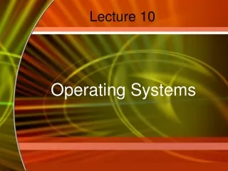
9. The Case of a Finite Queue Size Previously, we assumed that the queue could be arbitrarily large (infinite queue capacity). Now, we will address the somewhat more realistic problem in which there is a limit to the number of waiting customers (i.e. a finite queue capacity). Some preliminary assumptions should be addressed. First, we want to consider only those customers that enter the system to contribute to the customer arrival rate. We will assume that any customers appearing when the queue is full will go away. (More on this later.) Next, we will assume that the system capacity is N, meaning the maximum number of customers in the system, both waiting and being served. Therefore, for a single-stage, single-server system, the queue capacity will be N-1. la m L

10. The Case of a Finite Queue Size Previously, we assumed that the queue could be arbitrarily large (infinite queue capacity). Now, we will address the somewhat more realistic problem in which there is a limit to the number of waiting customers (i.e. a finite queue capacity). Some preliminary assumptions should be addressed. First, we want to consider only those customers that enter the system to contribute to the customer arrival rate. We will assume that any customers appearing when the queue is full will go away. Next, we will assume that the system capacity is N, meaning the maximum number of customers in the system, both waiting and being served. Therefore, for a single-stage, single-server system, the queue capacity will be N-1. la m L

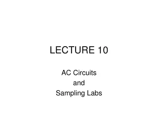
11. Back to the Balance Equations We start our analysis of finite capacity queueing systems with a return to the balance equations. Again we define the state of the system by the number of customers in the system. (10) . . . S0 S1 S2 SN-1 SN

12. More Scary Math As before we can develop a recurrence relation to express all proportions Pn in terms of P0. (11) and since SPn=1, we have (12) gives, Using the series identity, (13) (14) By substituting Equation (14) back into Equation (11) we obtain, (15)

13. A New L and W Since our queue size is finite, we do not have to ensure that the service rate exceed the arrival rate to maintain a steady-state condition. The customers that arrive when the queue is full, just go away. As before, the average number of customers in the system L is given by the number of customers in each state times the proportion of time the system is in each state. which you may wish to verify is equivalent to, and even more algebra fun reveals that

14. A Smaller l We need to be careful about what we mean by our arrival ratel. Since the rate includes some customers that never enter the system, we will have to reduce our effective arrival rate by the number of customers that go away. The proportion of customers that go away is equal to the proportion that arrive when the system is full, or PN. The rate at which customers actually enter the system is, therefore, le = l(1-PN )