Download
1 / 22
270 likes | 308 Vues
PETROPHYSICS: ROCK/LOG/SEISMIC CALIBRATION. John T. Kulha Petrophysical Consultant July 2016. Petrophysical Evaluation. Petrophysics: data acquisition. Acquire digital log files in LAS format lithology: spontaneous potential, gamma ray resistivity: normal, lateral, induction

E N D
PETROPHYSICS: ROCK/LOG/SEISMICCALIBRATION John T. Kulha Petrophysical Consultant July 2016
Petrophysics: data acquisition • Acquire digital log files in LAS format • lithology: spontaneous potential, gamma ray • resistivity: normal, lateral, induction • porosity: density, neutron, compressional and shear acoustic • others: caliper, microlog, cased-hole gamma ray/neutron, LWD/MWD, images, NMR • Review paper copy log data • verification of digital data • additions to existing digital data base (microlog, etc) • Acquire paper/digital copy of hydrocarbon logs • ROP, TG and CG curves; description of shows (fluorescence, cut, odor, etc); lithology • Rock data from multiple sources; petrophysical measurments
Petrophysics: data preparation • Build continuous digital file of all log curves in measured depth • LAS files (LIS, DLIS, ASCII) • digitize or scan to infill any missing data • Enter log header and log run information • mud parameters (weight, resistivities) • maximum temperature • Enter paleontological, geological correlation markers, perforations, test and core intervals • annotations of test results, production, core description, etc • Enter core data into digital log file • porosity, permeability, grain density, fluid saturations, etc
Petrophysics: data preparation • Perform selected edits of invalid data • “hand” edits (between runs, casing points, obvious bad data) • edits using similar response curves (conductivity) • edits using synthetic curves (acoustic or density) • Depth merge log curves to resistivity • porosity (neutron, bulk density, sonic) • lithology (gamma ray, spontaneous potential) • depth correlation between neutron and bulk density! • Enter directional information and perform TVD calculations (if applicable)
Petrophysics: data preparation • Perform environmental corrections and conversions • borehole and mud weight to gamma ray • matrix conversion to neutron • bulk density/density porosity • shift spontaneous potential to a constant shale baseline • resistivity invasion • Normalization of key log curves • neutron, bulk density and acoustic, gamma ray • only if reasonable data coverage and distribution exists • consistent “normalization” lithology interval in all wells • review quality of resistivity (“strange profiles”) • consistency in regional shales and/or other lithologies
Petrophysics: model development • Determine shale volume for clastic and carbonate reservoirs using single curve and x-plot indicators • SP, gamma ray, neutron, bulk density, resistivity • neutron-density, neutron-sonic and sonic-density crossplots • average value for final shale volume • minimum value for final shale volume • calibrate to X-ray diffraction or other core-derived clay measurements • compare final composite shale volume curve to individual components • gamma ray and/or neutron-bulk density better in carbonates • calibrate with geological model • Use to calculate “effective” from total porosity
Petrophysics: model development • Determine total porosity • matrix porosity (macro- and micro-porosity) • secondary porosity: fracture, vugular • correct to effective porosity • Multiple porosity tools • compensated neutron log and bulk density (PHIND) • compensated neutron log and acoustic (PHINS) • compare PHIND with PHINS • compare acoustic and PHIND for secondary porosity • Single or two porosity tools • compensated neutron log and the bulk density (PHIND) • compensated neutron log and acoustic (PHINS) • acoustic or density (PHIS, PHID)
Petrophysics: model development • Parameter selection (Rw, m, n, CEC, Qv, Rsh) • Formation water resistivity (Rw) • produced water: wireline, DST’s, intial tests or production • offset wells • water salinity catalogues • analysis of spontaneous potential, need mud filtrate resistivity value (Rmf) • Rw and cementation exponent (m): Pickett crossplot • total porosity versus resistivity (log-log crossplot) • apply in wet reservoirs; hydrocarbons won’t define Rw
Petrophysics: model development • Special core analysis for cementation (m) and saturation (n) exponents • rock catalogues with analogous rock types • empirical relationships • estimated from cuttings • Clay electrical properties for cation-exchange capacity water saturation model • clay type, amount and mode of distribution • analytical measurements • empirical relationships • Log-derived shale properties for shale volume water saturation model • clay type and mode of distribution • average log values in adjacent or internal shales
Petrophysics: model development • Water saturation calculation (Archie model) • resistivity from deepest investigating curve (invasion?) • total porosity • formation water resistivity, Rw • cementation, m, and saturation, n, exponents • Water saturation calculation (shale volume models) • Modified Simandoux, Indonesian, others • resistivity from deepest investigating curve (invasion?) • effective porosity (shale values RHOB, NPHI, DT) • shale volume, porosity and resistivity • formation water resistivity, Rw • cementation, m, and saturation, n, exponents
Petrophysics: model development • Water saturation calculation (cation-exchange capacity models) • Waxman-Smits, Dual Water (rigorous or simplified) • resistivity from deepest investigating curve (invasion?) • total porosity • cation exchange capacity • equivalent conductance • specific clay area • bound water resistivity • formation water resistivity • cementation, m (m*), and saturation, n (n*), exponents • shale volume and porosity
Petrophysics: model development • Pay distribution and reservoir properties are defined by cutoffs of key log curves • porosity • water saturation • shale volume • other curves, as needed (hydrocarbon pore volume, perm) • Cutoffs should be calibrated • producing intervals in wells • intervals that produce water • analogue data • consistent with permeability estimation • Reservoir property summation used in geological model, simulation, reserves and completion design
Rock/Log/Seismic Calibration-1 • Relationships between “rocks/logs/seismic” • rocks/logs/seismic must be calibrated to provide a complimentary and realistic geoscience and engineering evaluation • petrophysics and “petro-geophysics” • Rocks and logs • logs calibrated to rock type/reservoir quality • standard petrophysical relationships • porosity, water saturation, reservoir quality, permeability, pay • Rocks and seismic • seismic calibrated to rock type/reservoir quality • elastic variables • velocity, bulk density, acoustic impedance • Logs and seismics • seismic “calibrated” to corrected logs (rock type/reservoir quality) • synthetic elastic logs • lithology and fluid models • synthetic seismograms
PETROPHYSICAL RELATIONSHIPS SYNTHETIC SEISMOGRAMS SYNTHESIZED ELASTIC LOGS SEISMIC LOGS ROCKS Rock/Log/Seismic Calibration-2 ELASTIC VARIABLES VARIABLES SYNTHESIZED LOG TRANSFORM CALIBRATION MODEL ROCK/FLUID DISTRIBUTION TIME/DEPTH SEISMIC SIGNATURE AVO CALIBRATION
Rock/Log/Seismic Calibration-3 • Recorded acoustic and bulk density logs • inaccurate: miscalibration, erroneous tool response, service company problems • incomplete: intervals not logged, data not recorded, data lost • unavailable: logs not run, data lost, old wells (pre-sonic and bulk density) • Synthetic acoustic and bulk density logs • generated from resistivity/conductivity (primary independent variable) • generated from shale volume (secondary independent variable) • generated as a function of depth, rock type, correlation interval, geologic age, pressure regime (tertiary independent variables) • applied a common regression algorithm to a maximum number of wells within a project area • Problems resolved by synthetic logs • borehole rugosity and erroneous measurements • effects of borehole alteration due to drilling fluid reaction and stress relief • different service companies’ tools and associated tool response variations • tool miscalibration; wrong log scales (paper logs) • incomplete or unavailable logs
Rock/Log/Seismic Calibration-4 • Synthetic logs for in-situ conditions • effects of lithology and rock type change • wet reservoir response • hydrocarbon response • identify intervals of questionable measured data • Synthetic logs for modeled conditions • changes in lithology or reservoir quality • hydrocarbon fluid substitution • variations in reservoir quality and fluid content • Synthetic seismograms from synthetic logs • consistent character within a project area • provide usable well/seismic tie • provide synthetics where log data in not available or unusable
Rock/Log/Seismic Calibration-5 • Correlate intervals of similar rock properties • rock properties related to wireline log responses • guided by regional depositional model and environments • guided by regional seismic correlation with preliminary log/seismic tie • incorporate mudlog lithology and/or independent cuttings descriptions • “overlook” intervals of questionable or missing log data • Create shale volume curve • lithology related wireline logs • gamma ray, spontaneous potential, neutron/density, resistivity • defined by either reservoir scale or seismic scale • flexible to accommodate changes in lithology • Build calibration data set • select intervals of acceptable measured log data • “experience” driven and supplemented with other discipline input • representative of all various independent variables • inclusive of multiple well data sets
Rock/Log/Seismic Calibration-6 • Perform multivariable regression and calculate synthetic logs • shale volume (VSH) log • resistivity (RT) or conductivity (COND) log • Other log curves, NPHI, PE, mudlog curves(?) • depth, geologic age, depositional environment, pressure regime • regression coefficients, A1, A2, A3, A4 • RHOB=A1+A2*(VSH)+A3*(LOG (RT), COND)+A4*(DEPT) • DT=A1+A2*(LF, VSH)+A3*(LOG (RT), COND)+A4*(DEPT) • may simplify to only two variables • Compare synthetic logs with calibration data set • modify calibration intervals, other independent variables • repeat process until correlation with measured data or tie to seismic is acceptable • Perform fluid substitution or calibrate directly • calibrate directly to in-situ fluid conditions • calculate wet reservoir condition and then substitute hydrocarbons • selected intervals from representative wells
Example well: 4 intervals 2950’- 4000’ 4400’- 5400’ T1: SP-blue; GR-black, VSH-red T2: RD-red; RM-green T3: RHOB-black; RHOB-ED, red; CALI-green T4: DT-black; DT-ED-red Yellow shading indicates amount of error between measured and synthetic (corrected) log curve 8100’- 9750’ 6100’- 7600’