Download
1 / 75
770 likes | 909 Vues
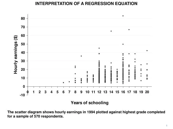
INTERPRETATION OF A REGRESSION EQUATION. The scatter diagram shows hourly earnings in 1994 plotted against highest grade completed for a sample of 570 respondents. 1. INTERPRETATION OF A REGRESSION EQUATION. . reg EARNINGS S

E N D
INTERPRETATION OF A REGRESSION EQUATION The scatter diagram shows hourly earnings in 1994 plotted against highest grade completed for a sample of 570 respondents. 1
INTERPRETATION OF A REGRESSION EQUATION . reg EARNINGS S Source | SS df MS Number of obs = 570 ---------+------------------------------ F( 1, 568) = 65.64 Model | 3977.38016 1 3977.38016 Prob > F = 0.0000 Residual | 34419.6569 568 60.5979875 R-squared = 0.1036 ---------+------------------------------ Adj R-squared = 0.1020 Total | 38397.0371 569 67.4816117 Root MSE = 7.7845 ------------------------------------------------------------------------------ EARNINGS | Coef. Std. Err. t P>|t| [95% Conf. Interval] ---------+-------------------------------------------------------------------- S | 1.073055 .1324501 8.102 0.000 .8129028 1.333206 _cons | -1.391004 1.820305 -0.764 0.445 -4.966354 2.184347 ------------------------------------------------------------------------------ This is the output from a regression of earnings on highest grade completed, using Stata. 4
INTERPRETATION OF A REGRESSION EQUATION . reg EARNINGS S Source | SS df MS Number of obs = 570 ---------+------------------------------ F( 1, 568) = 65.64 Model | 3977.38016 1 3977.38016 Prob > F = 0.0000 Residual | 34419.6569 568 60.5979875 R-squared = 0.1036 ---------+------------------------------ Adj R-squared = 0.1020 Total | 38397.0371 569 67.4816117 Root MSE = 7.7845 ------------------------------------------------------------------------------ EARNINGS | Coef. Std. Err. t P>|t| [95% Conf. Interval] ---------+-------------------------------------------------------------------- S | 1.073055 .1324501 8.102 0.000 .8129028 1.333206 _cons | -1.391004 1.820305 -0.764 0.445 -4.966354 2.184347 ------------------------------------------------------------------------------ For the time being, we will be concerned only with the estimates of the parameters. The variables in the regression are listed in the first column and the second column gives the estimates of their coefficients. 5
INTERPRETATION OF A REGRESSION EQUATION . reg EARNINGS S Source | SS df MS Number of obs = 570 ---------+------------------------------ F( 1, 568) = 65.64 Model | 3977.38016 1 3977.38016 Prob > F = 0.0000 Residual | 34419.6569 568 60.5979875 R-squared = 0.1036 ---------+------------------------------ Adj R-squared = 0.1020 Total | 38397.0371 569 67.4816117 Root MSE = 7.7845 ------------------------------------------------------------------------------ EARNINGS | Coef. Std. Err. t P>|t| [95% Conf. Interval] ---------+-------------------------------------------------------------------- S | 1.073055 .1324501 8.102 0.000 .8129028 1.333206 _cons | -1.391004 1.820305 -0.764 0.445 -4.966354 2.184347 ------------------------------------------------------------------------------ In this case there is only one variable, S, and its coefficient is 1.073. _cons, in Stata, refers to the constant. The estimate of the intercept is -1.391. 6
INTERPRETATION OF A REGRESSION EQUATION ^ Here is the scatter diagram again, with the regression line shown. 7
INTERPRETATION OF A REGRESSION EQUATION ^ What do the coefficients actually mean? 8
INTERPRETATION OF A REGRESSION EQUATION ^ To answer this question, you must refer to the units in which the variables are measured. 9
INTERPRETATION OF A REGRESSION EQUATION ^ S is measured in years (strictly speaking, grades completed), EARNINGS in dollars per hour. So the slope coefficient implies that hourly earnings increase by $1.07 for each extra year of schooling. 10
INTERPRETATION OF A REGRESSION EQUATION ^ We will look at a geometrical representation of this interpretation. To do this, we will enlarge the marked section of the scatter diagram. 11
INTERPRETATION OF A REGRESSION EQUATION $11.49 $1.07 One year $10.41 The regression line indicates that completing 12th grade instead of 11th grade would increase earnings by $1.073, from $10.413 to $11.486, as a general tendency. 12
INTERPRETATION OF A REGRESSION EQUATION ^ You should ask yourself whether this is a plausible figure. If it is implausible, this could be a sign that your model is misspecified in some way. 13
INTERPRETATION OF A REGRESSION EQUATION ^ For low levels of education it might be plausible. But for high levels it would seem to be an underestimate. 14
INTERPRETATION OF A REGRESSION EQUATION ^ What about the constant term? (Try to answer this question yourself before continuing with this sequence.) 15
INTERPRETATION OF A REGRESSION EQUATION ^ Literally, the constant indicates that an individual with no years of education would have to pay $1.39 per hour to be allowed to work. 16
INTERPRETATION OF A REGRESSION EQUATION ^ This does not make any sense at all, an interpretation of negative payment is impossible to sustain. 17
INTERPRETATION OF A REGRESSION EQUATION ^ A safe solution to the problem is to limit the interpretation to the range of the sample data, and to refuse to extrapolate on the ground that we have no evidence outside the data range. 18
INTERPRETATION OF A REGRESSION EQUATION ^ With this explanation, the only function of the constant term is to enable you to draw the regression line at the correct height on the scatter diagram. It has no meaning of its own. 19
MULTIPLE REGRESSION WITH TWO EXPLANATORY VARIABLES: EXAMPLE EARNINGS = b1+ b2S + b3A+ u Specifically, we will look at an earnings function model where hourly earnings, EARNINGS, depend on years of schooling (highest grade completed), S, and a measure of cognitive ability, A. The model has three dimensions, one each for EARNINGS, S, and A. The starting point for investigating the determination of EARNINGS is the intercept, b1. Literally the intercept gives EARNINGS for those respondents who have no schooling and who scored zero on the ability test. However, the ability score is scaled in such a way as to make it impossible to score zero. Hence a literal interpretation of b1 would be unwise. The next term on the right side of the equation gives the effect of variations in S. A one year increase in S causes EARNINGS to increase by b2 dollars, holding A constant. Similarly, the third term gives the effect of variations in A. A one point increase in A causes earnings to increase by b3 dollars, holding S constant. The final element of the model is the disturbance term, u. In this observation, u happens to have a positive value. 2
MULTIPLE REGRESSION WITH TWO EXPLANATORY VARIABLES: EXAMPLE A sample consists of a number of observations generated in this way. Note that the interpretation of the model does not depend on whether S and A are correlated or not. However we do assume that the effects of S and A on EARNINGS are additive. The impact of a difference in S on EARNINGS is not affected by the value of A, or vice versa. The regression coefficients are derived using the same least squares principle used in simple regression analysis. The fitted value of Y in observation i depends on our choice of b1, b2, and b3. 11
MULTIPLE REGRESSION WITH TWO EXPLANATORY VARIABLES: EXAMPLE The residual ei in observation i is the difference between the actual and fitted values of Y. 12
MULTIPLE REGRESSION WITH TWO EXPLANATORY VARIABLES: EXAMPLE We define RSS, the sum of the squares of the residuals, and choose b1, b2, and b3 so as to minimize it. 13
MULTIPLE REGRESSION WITH TWO EXPLANATORY VARIABLES: EXAMPLE . reg EARNINGS S ASVABC Source | SS df MS Number of obs = 570 ---------+------------------------------ F( 2, 567) = 39.98 Model | 4745.74965 2 2372.87483 Prob > F = 0.0000 Residual | 33651.2874 567 59.3497133 R-squared = 0.1236 ---------+------------------------------ Adj R-squared = 0.1205 Total | 38397.0371 569 67.4816117 Root MSE = 7.7039 ------------------------------------------------------------------------------ EARNINGS | Coef. Std. Err. t P>|t| [95% Conf. Interval] ---------+-------------------------------------------------------------------- S | .7390366 .1606216 4.601 0.000 .4235506 1.054523 ASVABC | .1545341 .0429486 3.598 0.000 .0701764 .2388918 _cons | -4.624749 2.0132 -2.297 0.022 -8.578989 -.6705095 ------------------------------------------------------------------------------ Here is the regression output for the earnings function using Data Set 21. 19
MULTIPLE REGRESSION WITH TWO EXPLANATORY VARIABLES: EXAMPLE . reg EARNINGS S A Source | SS df MS Number of obs = 570 ---------+------------------------------ F( 2, 567) = 39.98 Model | 4745.74965 2 2372.87483 Prob > F = 0.0000 Residual | 33651.2874 567 59.3497133 R-squared = 0.1236 ---------+------------------------------ Adj R-squared = 0.1205 Total | 38397.0371 569 67.4816117 Root MSE = 7.7039 ------------------------------------------------------------------------------ EARNINGS | Coef. Std. Err. t P>|t| [95% Conf. Interval] ---------+-------------------------------------------------------------------- S | .7390366 .1606216 4.601 0.000 .4235506 1.054523 A | .1545341 .0429486 3.598 0.000 .0701764 .2388918 _cons | -4.624749 2.0132 -2.297 0.022 -8.578989 -.6705095 ------------------------------------------------------------------------------ It indicates that earnings increase by $0.74 for every extra year of schooling and by $0.15 for every extra point increase in A. 20
MULTIPLE REGRESSION WITH TWO EXPLANATORY VARIABLES: EXAMPLE . reg EARNINGS S A Source | SS df MS Number of obs = 570 ---------+------------------------------ F( 2, 567) = 39.98 Model | 4745.74965 2 2372.87483 Prob > F = 0.0000 Residual | 33651.2874 567 59.3497133 R-squared = 0.1236 ---------+------------------------------ Adj R-squared = 0.1205 Total | 38397.0371 569 67.4816117 Root MSE = 7.7039 ------------------------------------------------------------------------------ EARNINGS | Coef. Std. Err. t P>|t| [95% Conf. Interval] ---------+-------------------------------------------------------------------- S | .7390366 .1606216 4.601 0.000 .4235506 1.054523 A | .1545341 .0429486 3.598 0.000 .0701764 .2388918 _cons | -4.624749 2.0132 -2.297 0.022 -8.578989 -.6705095 ------------------------------------------------------------------------------ Literally, the intercept indicates that an individual who had no schooling and an A score of zero would have hourly earnings of -$4.62. 21
MULTIPLE REGRESSION WITH TWO EXPLANATORY VARIABLES: EXAMPLE . reg EARNINGS S A Source | SS df MS Number of obs = 570 ---------+------------------------------ F( 2, 567) = 39.98 Model | 4745.74965 2 2372.87483 Prob > F = 0.0000 Residual | 33651.2874 567 59.3497133 R-squared = 0.1236 ---------+------------------------------ Adj R-squared = 0.1205 Total | 38397.0371 569 67.4816117 Root MSE = 7.7039 ------------------------------------------------------------------------------ EARNINGS | Coef. Std. Err. t P>|t| [95% Conf. Interval] ---------+-------------------------------------------------------------------- S | .7390366 .1606216 4.601 0.000 .4235506 1.054523 A | .1545341 .0429486 3.598 0.000 .0701764 .2388918 _cons | -4.624749 2.0132 -2.297 0.022 -8.578989 -.6705095 ------------------------------------------------------------------------------ Obviously, this is impossible. The lowest value of S in the sample was 6, and the lowest A score was 22. We have obtained a nonsense estimate because we have extrapolated too far from the data range. 22
t TEST OF A HYPOTHESIS RELATING TO A REGRESSION COEFFICIENT t Distribution: Critical values of t Degrees of Two-tailed test 10% 5% 2% 1% 0.2% 0.1% freedom One-tailed test 5% 2.5% 1% 0.5% 0.1% 0.05% 1 6.314 12.706 31.821 63.657 318.31 636.62 2 2.920 4.303 6.965 9.925 22.327 31.598 3 2.353 3.182 4.541 5.841 10.214 12.924 4 2.132 2.776 3.747 4.604 7.173 8.610 5 2.015 2.571 3.365 4.032 5.893 6.869 … … … … … … … … … … … … … … 18 1.734 2.101 2.552 2.878 3.610 3.922 19 1.729 2.093 2.539 2.861 3.579 3.883 20 1.725 2.086 2.528 2.845 3.552 3.850 … … … … … … … … … … … … … … 120 1.658 1.980 2.358 2.617 3.160 3.373 1.645 1.960 2.326 2.576 3.090 3.291 For this reason we need to refer to a table of critical values of t when performing significance tests on the coefficients of a regression equation. 18
t TEST OF A HYPOTHESIS RELATING TO A REGRESSION COEFFICIENT t Distribution: Critical values of t Degrees of Two-tailed test 10% 5% 2% 1% 0.2% 0.1% freedom One-tailed test 5% 2.5% 1% 0.5% 0.1% 0.05% 1 6.314 12.706 31.821 63.657 318.31 636.62 2 2.920 4.303 6.965 9.925 22.327 31.598 3 2.353 3.182 4.541 5.841 10.214 12.924 4 2.132 2.776 3.747 4.604 7.173 8.610 5 2.015 2.571 3.365 4.032 5.893 6.869 … … … … … … … … … … … … … … 18 1.734 2.101 2.552 2.878 3.610 3.922 19 1.729 2.093 2.539 2.861 3.579 3.883 20 1.725 2.086 2.528 2.845 3.552 3.850 … … … … … … … … … … … … … … 120 1.658 1.980 2.358 2.617 3.160 3.373 1.645 1.960 2.326 2.576 3.090 3.291 At the top of the table are listed possible significance levels for a test. For the time being we will be performing two-tailed tests, so ignore the line for one-tailed tests. 19
t TEST OF A HYPOTHESIS RELATING TO A REGRESSION COEFFICIENT t Distribution: Critical values of t Degrees of Two-tailed test 10% 5% 2% 1% 0.2% 0.1% freedom One-tailed test 5% 2.5% 1% 0.5% 0.1% 0.05% 1 6.314 12.706 31.821 63.657 318.31 636.62 2 2.920 4.303 6.965 9.925 22.327 31.598 3 2.353 3.182 4.541 5.841 10.214 12.924 4 2.132 2.776 3.747 4.604 7.173 8.610 5 2.015 2.571 3.365 4.032 5.893 6.869 … … … … … … … … … … … … … … 18 1.734 2.101 2.552 2.878 3.610 3.922 19 1.729 2.093 2.539 2.861 3.579 3.883 20 1.725 2.086 2.528 2.845 3.552 3.850 … … … … … … … … … … … … … … 120 1.658 1.980 2.358 2.617 3.160 3.373 1.645 1.960 2.326 2.576 3.090 3.291 Hence if we are performing a (two-tailed) 5% significance test, we should use the column thus indicated in the table. 20
t TEST OF A HYPOTHESIS RELATING TO A REGRESSION COEFFICIENT t Distribution: Critical values of t Degrees of Two-tailed test 10% 5% 2% 1% 0.2% 0.1% freedom One-tailed test 5% 2.5% 1% 0.5% 0.1% 0.05% 1 6.314 12.706 31.821 63.657 318.31 636.62 2 2.920 4.303 6.965 9.925 22.327 31.598 3 2.353 3.182 4.541 5.841 10.214 12.924 4 2.132 2.776 3.747 4.604 7.173 8.610 5 2.015 2.571 3.365 4.032 5.893 6.869 … … … … … … … … … … … … … … 18 1.734 2.101 2.552 2.878 3.610 3.922 19 1.729 2.093 2.539 2.861 3.579 3.883 20 1.725 2.086 2.528 2.845 3.552 3.850 … … … … … … … … … … … … … … 120 1.658 1.980 2.358 2.617 3.160 3.373 1.645 1.960 2.326 2.576 3.090 3.291 Number of degrees of freedom in a regression = number of observations - number of parameters estimated. The left hand vertical column lists degrees of freedom. The number of degrees of freedom in a regression is defined to be the number of observations minus the number of parameters estimated. 21
t TEST OF A HYPOTHESIS RELATING TO A REGRESSION COEFFICIENT t Distribution: Critical values of t Degrees of Two-tailed test 10% 5% 2% 1% 0.2% 0.1% freedom One-tailed test 5% 2.5% 1% 0.5% 0.1% 0.05% 1 6.314 12.706 31.821 63.657 318.31 636.62 2 2.920 4.303 6.965 9.925 22.327 31.598 3 2.353 3.182 4.541 5.841 10.214 12.924 4 2.132 2.776 3.747 4.604 7.173 8.610 5 2.015 2.571 3.365 4.032 5.893 6.869 … … … … … … … … … … … … … … 18 1.734 2.101 2.552 2.878 3.610 3.922 19 1.729 2.093 2.539 2.861 3.579 3.883 20 1.725 2.086 2.528 2.845 3.552 3.850 … … … … … … … … … … … … … … 120 1.658 1.980 2.358 2.617 3.160 3.373 1.645 1.960 2.326 2.576 3.090 3.291 In a simple regression, we estimate just two parameters, the constant and the slope coefficient, so the number of degrees of freedom is n - 2 if there are n observations. 22
t TEST OF A HYPOTHESIS RELATING TO A REGRESSION COEFFICIENT t Distribution: Critical values of t Degrees of Two-tailed test 10% 5% 2% 1% 0.2% 0.1% freedom One-tailed test 5% 2.5% 1% 0.5% 0.1% 0.05% 1 6.314 12.706 31.821 63.657 318.31 636.62 2 2.920 4.303 6.965 9.925 22.327 31.598 3 2.353 3.182 4.541 5.841 10.214 12.924 4 2.132 2.776 3.747 4.604 7.173 8.610 5 2.015 2.571 3.365 4.032 5.893 6.869 … … … … … … … … … … … … … … 18 1.734 2.101 2.552 2.878 3.610 3.922 19 1.729 2.093 2.539 2.861 3.579 3.883 20 1.725 2.086 2.528 2.845 3.552 3.850 … … … … … … … … … … … … … … 120 1.658 1.980 2.358 2.617 3.160 3.373 1.645 1.960 2.326 2.576 3.090 3.291 If we were performing a regression with 20 observations, as in the price inflation/wage inflation example, the number of degrees of freedom would be 18 and the critical value of t for a 5% test would be 2.101. 23
t TEST OF A HYPOTHESIS RELATING TO A REGRESSION COEFFICIENT t Distribution: Critical values of t Degrees of Two-tailed test 10% 5% 2% 1% 0.2% 0.1% freedom One-tailed test 5% 2.5% 1% 0.5% 0.1% 0.05% 1 6.314 12.706 31.821 63.657 318.31 636.62 2 2.920 4.303 6.965 9.925 22.327 31.598 3 2.353 3.182 4.541 5.841 10.214 12.924 4 2.132 2.776 3.747 4.604 7.173 8.610 5 2.015 2.571 3.365 4.032 5.893 6.869 … … … … … … … … … … … … … … 18 1.734 2.101 2.552 2.878 3.610 3.922 19 1.729 2.093 2.539 2.861 3.579 3.883 20 1.725 2.086 2.528 2.845 3.552 3.850 … … … … … … … … … … … … … … 120 1.658 1.980 2.358 2.617 3.160 3.373 1.645 1.960 2.326 2.576 3.090 3.291 Note that as the number of degrees of freedom becomes large, the critical value converges on 1.96, the critical value for the normal distribution. This is because the t distribution converges on the normal distribution. 24
t TEST OF A HYPOTHESIS RELATING TO A REGRESSION COEFFICIENT t Distribution: Critical values of t Degrees of Two-tailed test 10% 5% 2% 1% 0.2% 0 .1% freedom One-tailed test 5% 2.5% 1% 0.5% 0.1% 0.05% 1 6.314 12.706 31.821 63.657 318.31 636.62 2 2.920 4.303 6.965 9.925 22.327 31.598 3 2.353 3.182 4.541 5.841 10.214 12.924 4 2.132 2.776 3.747 4.604 7.173 8.610 5 2.015 2.571 3.365 4.032 5.893 6.869 … … … … … … … … … … … … … … 18 1.734 2.101 2.552 2.878 3.610 3.922 19 1.729 2.093 2.539 2.861 3.579 3.883 20 1.725 2.086 2.528 2.845 3.552 3.850 … … … … … … … … … … … … … … 120 1.658 1.980 2.358 2.617 3.160 3.373 1.645 1.960 2.326 2.576 3.090 3.291 If instead we wished to perform a 1% significance test, we would use the column indicated above. Note that as the number of degrees of freedom becomes large, the critical value converges to 2.58, the critical value for the normal distribution. 27
t TEST OF A HYPOTHESIS RELATING TO A REGRESSION COEFFICIENT t Distribution: Critical values of t Degrees of Two-tailed test 10% 5% 2% 1% 0.2% 0 .1% freedom One-tailed test 5% 2.5% 1% 0.5% 0.1% 0.05% 1 6.314 12.706 31.821 63.657 318.31 636.62 2 2.920 4.303 6.965 9.925 22.327 31.598 3 2.353 3.182 4.541 5.841 10.214 12.924 4 2.132 2.776 3.747 4.604 7.173 8.610 5 2.015 2.571 3.365 4.032 5.893 6.869 … … … … … … … … … … … … … … 18 1.734 2.101 2.552 2.878 3.610 3.922 19 1.729 2.093 2.539 2.861 3.579 3.883 20 1.725 2.086 2.528 2.845 3.552 3.850 … … … … … … … … … … … … … … 120 1.658 1.980 2.358 2.617 3.160 3.373 1.645 1.960 2.326 2.576 3.090 3.291 For a simple regression with 20 observations, the critical value of t at the 1% level is 2.878. 28
t TEST OF A HYPOTHESIS RELATING TO A REGRESSION COEFFICIENT s.d. of b2 known s.d. of b2 not known discrepancy between hypothetical value and sample estimate, in terms of s.d.: discrepancy between hypothetical value and sample estimate, in terms of s.e.: 5% significance test: reject H0: b2 = b2 if z > 1.96 or z < -1.96 1% significance test: reject H0: b2 = b2 if t > 2.878 or t < -2.878 0 0 So we should this figure in the test procedure for a 1% test. 29
EXERCISE 3.10 A researcher with a sample of 50 individuals with similar education but differing amounts of training hypothesizes that hourly earnings, EARNINGS, may be related to hours of training, TRAINING, according to the relationship EARNINGS = b1 + b2TRAINING + u He is prepared to test the null hypothesis H0: b2 = 0 against the alternative hypothesis H1: b2 0 at the 5 percent and 1 percent levels. What should he report 1. If b2 = 0.30, s.e.(b2) = 0.12? 2. If b2 = 0.55, s.e.(b2) = 0.12? 3. If b2 = 0.10, s.e.(b2) = 0.12? 4. If b2 = -0.27, s.e.(b2) = 0.12? 1
EXERCISE EARNINGS = b1 + b2TRAINING + u H0: b2 = 0, H1: b2 0 n = 50, so 48 degrees of freedom There are 50 observations and 2 parameters have been estimated, so there are 48 degrees of freedom. 2
EXERCISE EARNINGS = b1 + b2TRAINING + u H0: b2 = 0, H1: b2 0 n = 50, so 48 degrees of freedom tcrit, 5% = 2.01, tcrit, 1% = 2.68 The table giving the critical values of t does not give the values for 48 degrees of freedom. We will use the values for 50 as a guide. For the 5% level the value is 2.01, and for the 1% level it is 2.68. The critical values for 48 will be slightly higher. 3
EXERCISE EARNINGS = b1 + b2TRAINING + u H0: b2 = 0, H1: b2 0 n = 50, so 48 degrees of freedom tcrit, 5% = 2.01, tcrit, 1% = 2.68 _______________________________________________ 1. If b2 = 0.30, s.e.(b2) = 0.12? t = 2.50. In the first case, the t statistic is 2.50. 4
EXERCISE EARNINGS = b1 + b2TRAINING + u H0: b2 = 0, H1: b2 0 n = 50, so 48 degrees of freedom tcrit, 5% = 2.01, tcrit, 1% = 2.68 _______________________________________________ 1. If b2 = 0.30, s.e.(b2) = 0.12? t = 2.50. Reject H0 at the 5% level but not at the 1% level. This is greater than the critical value of t at the 5% level, but less than the critical value at the 1% level. 5
EXERCISE EARNINGS = b1 + b2TRAINING + u H0: b2 = 0, H1: b2 0 n = 50, so 48 degrees of freedom tcrit, 5% = 2.01, tcrit, 1% = 2.68 _______________________________________________ 1. If b2 = 0.30, s.e.(b2) = 0.12? t = 2.50. Reject H0 at the 5%, but not at the 1%, level. In this case we should mention both tests. It is not enough to say "Reject at the 5% level", because it leaves open the possibility that we might be able to reject at the 1% level. 6
EXERCISE EARNINGS = b1 + b2TRAINING + u H0: b2 = 0, H1: b2 0 n = 50, so 48 degrees of freedom tcrit, 5% = 2.01, tcrit, 1% = 2.68 _______________________________________________ 1. If b2 = 0.30, s.e.(b2) = 0.12? t = 2.50. Reject H0 at the 5%, but not at the 1%, level. Likewise it is not enough to say "Do not reject at the 1% level", because this does not reveal whether the result is significant at the 5% level or not. 7
EXERCISE EARNINGS = b1 + b2TRAINING + u H0: b2 = 0, H1: b2 0 n = 50, so 48 degrees of freedom tcrit, 5% = 2.01, tcrit, 1% = 2.68 _______________________________________________ 2. If b2 = 0.55, s.e.(b2) = 0.12? t = 4.58. In the second case, t is equal to 4.58. 8
EXERCISE EARNINGS = b1 + b2TRAINING + u H0: b2 = 0, H1: b2 0 n = 50, so 48 degrees of freedom tcrit, 5% = 2.01, tcrit, 1% = 2.68 _______________________________________________ 2. If b2 = 0.55, s.e.(b2) = 0.12? t = 4.58. Reject H0 at the 1% level. We report only the result of the 1% test. There is no need to mention the 5% test. If you do, you reveal that you do not understand that rejection at the 1% level automatically means rejection at the 5% level, and you look ignorant. 9
EXERCISE EARNINGS = b1 + b2TRAINING + u H0: b2 = 0, H1: b2 0 n = 50, so 48 degrees of freedom tcrit, 5% = 2.01, tcrit, 1% = 2.68 _______________________________________________ 2. If b2 = 0.55, s.e.(b2) = 0.12? t = 4.58. Reject H0 at the 0.1% level (tcrit, 0.1% = 3.50). Actually, given the large t statistic, it is a good idea to investigate whether we can reject H0 at the 0.1% level. It turns out that we can. The critical value for 50 degrees of freedom is 3.50. So we just report the outcome of this test. There is no need to mention the 1% test. 10
EXERCISE EARNINGS = b1 + b2TRAINING + u H0: b2 = 0, H1: b2 0 n = 50, so 48 degrees of freedom tcrit, 5% = 2.01, tcrit, 1% = 2.68 _______________________________________________ 2. If b2 = 0.55, s.e.(b2) = 0.12? t = 4.58. Reject H0 at the 0.1% level (tcrit, 0.1% = 3.50). Why is it a good idea to press on to a 0.1% test, if the t statistic is large? Try to answer this question before looking at the next slide. 11
EXERCISE 3.10 EARNINGS = b1 + b2TRAINING + u H0: b2 = 0, H1: b2 0 n = 50, so 48 degrees of freedom tcrit, 5% = 2.01, tcrit, 1% = 2.68 _______________________________________________ 2. If b2 = 0.55, s.e.(b2) = 0.12? t = 4.58. Reject H0 at the 0.1% level (tcrit, 0.1% = 3.50). The reason is that rejection at the 1% level still leaves open the possibility of a 1% risk of having made a Type I error (rejecting the null hypothesis when it is in fact true). So there is a 1% risk of the "significant" result having occurred as a matter of chance. 12
EXERCISE EARNINGS = b1 + b2TRAINING + u H0: b2 = 0, H1: b2 0 n = 50, so 48 degrees of freedom tcrit, 5% = 2.01, tcrit, 1% = 2.68 _______________________________________________ 2. If b2 = 0.55, s.e.(b2) = 0.12? t = 4.58. Reject H0 at the 0.1% level (tcrit, 0.1% = 3.50). If you can reject at the 0.1% level, you reduce that risk to one tenth of 1%. This means that the result is almost certainly genuine. 13
EXERCISE EARNINGS = b1 + b2TRAINING + u H0: b2 = 0, H1: b2 0 n = 50, so 48 degrees of freedom tcrit, 5% = 2.01, tcrit, 1% = 2.68 _______________________________________________ 3. If b2 = 0.10, s.e.(b2) = 0.12? t = 0.83. In the third case, t is equal to 0.83. 14
EXERCISE EARNINGS = b1 + b2TRAINING + u H0: b2 = 0, H1: b2 0 n = 50, so 48 degrees of freedom tcrit, 5% = 2.01, tcrit, 1% = 2.68 _______________________________________________ 3. If b2 = 0.10, s.e.(b2) = 0.12? t = 0.83. Do not reject H0 at the 5% level. We report only the result of the 5% test. There is no need to mention the 1% test. If you do, you reveal that you do not understand that not rejecting at the 5% level automatically means not rejecting at the 1% level, and you look ignorant. 15