Download
1 / 27
270 likes | 378 Vues
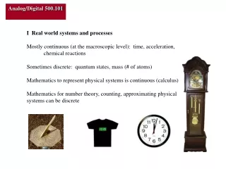
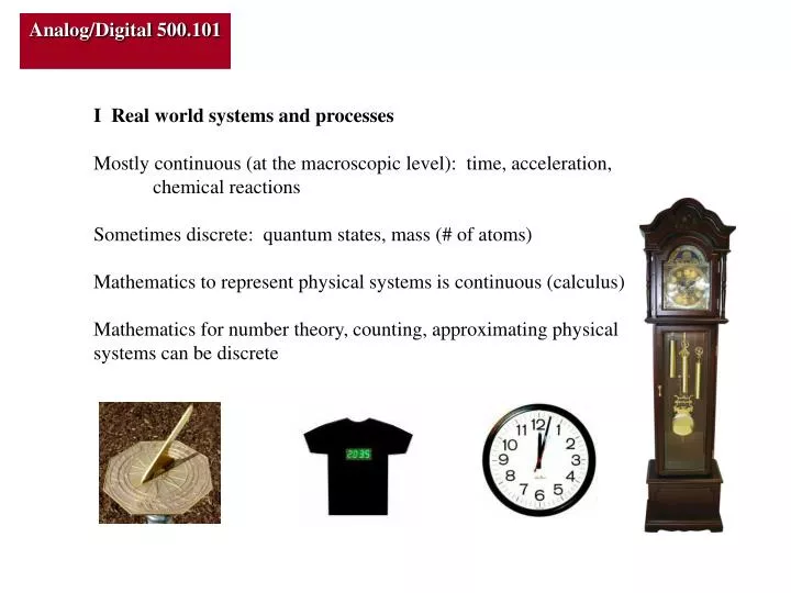
I Real world systems and processes Mostly continuous (at the macroscopic level): time, acceleration, chemical reactions Sometimes discrete: quantum states, mass (# of atoms) Mathematics to represent physical systems is continuous (calculus)

E N D
I Real world systems and processes Mostly continuous (at the macroscopic level): time, acceleration, chemical reactions Sometimes discrete: quantum states, mass (# of atoms) Mathematics to represent physical systems is continuous (calculus) Mathematics for number theory, counting, approximating physical systems can be discrete
II Representation of information • A. Continuous—represented analogously as a value of a continuously variable parameter • position of a needle on a meter • rotational angle of a gear • amount of water in a vessel • electric charge on a capacitor • B. Discrete—digitized as a set of discrete values corresponding to a finite number • of states • 1. digital clock • 2. painted pickets • 3. on/off, as a switch
III Representation of continuous processes • Analogous to the process itself • Great Brass Brain—a geared machine to simulate the tides • Slide rule—an instrument which does multiplication by adding lengths which correspond to the logarithms of numbers. • Differential analyzer (Vannevar Bush)—variable-size friction wheels to simulate the behavior of differential equations Vannevar Bush integrator Tide calculator
Brass Brain was the equal of 100 mathematicians, weighted a mere 2500 lbs Imagine the fearful gnashings of mathematicians in November, 1928 upon reading this account of the USGS's new "brass brain," which could "do the work of 100 trained mathematicians" in calculating tides: The machine weighs 2,500 pounds. It is 11 feet long, 2 feet wide, and 6 feet high. Its whirring cogs are enclosed in a housing of mahogany and glass. Earthquakes, fresh-water floods, and strong winds that cannot be predicted affect the accuracy of the Brass Brain to a degree. Nevertheless 70% of the predicted tides agree within five minutes of the observed tide. The Coast and Geodetic Survey issues an annual bulletin in which it lists the forthcoming tides in 84 ports of the world. The report contains upwards of a million figures, all compiled by the Brass Brain. It has been estimated that the Brass Brain saves the government $125,000 each year in salaries of mathematicians who would be required to take its place.
From Instruments of Science: an historical encyclopedia Great Brass Brain “It remained in use until the late 1960s,when an IBM 7090 computer took over the job. Even when digital computers finally took over from analog instruments, the amount of arithmetic needed to properly evaluate the cosine series was so vast that the output had to be limited to simply times of high and low tide for any particular area. This was overcome only when, during the 1970s, digital computers became powerful enough. . .”
Discrete representations What is it?? What is it?? What is it??
Electronic analog computers—circuitry connected to simulate differential equations • Phonograph record—wiggles in grooves to represent sound oscillations • Electric clocks • Mercury thermometers/barometers Stereo phonograph record
IV Manipulation A. Analog 1. adding the length-equivalents of logarithms to obtain a multiply, e.g., a slide-rule 2. adjusting the volume on a stereo 3. sliding a weight on a balance-beam scale 4. adding charge to an electrical capacitor B. Discrete 1. counting—push-button counters 2. digital operations—mechanical calculators 3. switching—open/closing relays 4. logic circuits—true/false determination Marble binary counter Marchant mechanical calculator
V Analog vs. Discrete Note: "Digital" is a form of representation for discrete A. Analog 1. infinitely variable--information density high 2. limited resolution--to what resolution can you read a meter? 3. irrecoverable data degradation--sandpaper a vinyl record B. Discrete/Digital 1. limited states--information density low, e.g., one decimal digit can represent only one of ten values 2. arbitrary resolution--keep adding states (or digits) 3. mostly recoverable data degradation, e.g., if information is encoded as painted/not-painted pickets, repainting can perfectly restore data
VI Digital systems A. decimal--not so good, because there are few 10-state devices that could be used to store information fingers. . .? B. binary--excellent for hardware; lots of 2-state devices: switches, lights, magnetics--poor for communication: 2-state devices require many digits to represent values with reasonable resolution--excellent for logic systems whose states are true and false. But binary is king because components are so easy (and cheap) to fabricate. C. octal --base 8: used to conveniently represent binary data; almost as efficient as decimal D. hexadecimal--base 16: more efficient than decimal; more practical than octal because of binary digit groupings in computers
VII Binary logic and arithmetic A. Background 1. George Boole(1854) linked arithmetic, logic, and binary number systems by showing how a binary system could be used to simplify complex logic problems 2. Claude Shannon(1938) demonstrated that any logic problem could be represented by a system of series and parallel switches; and that binary addition could be done with electric switches 3. Two branches of binary logic systems a) Combinatorial—in which the output depends only on the present state of the inputs b) Sequential—in which the output may depend on a previous state of the inputs, e.g., the “flip-flop” circuit
C AND gate A B A B C 0 0 0 1 0 0 0 1 0 1 1 1
C A B C Battery AND gate A B A B C 0 0 0 1 0 0 0 1 0 1 1 1 Simple “AND” Circuit
C A B OR gate A B C 0 0 0 1 0 1 0 1 1 1 1 1
C A B OR gate Simple “OR” circuit A B C 0 0 0 1 0 1 0 1 1 1 1 1 A B C
A B A B 1 0 0 1 NOT gate
A B A A B 1 0 0 1 B NOT gate Simple “NOT” circuit
C NAND gate A B A B C 0 0 1 1 0 1 0 1 1 1 1 0
C A B C Battery NAND gate A B A B C 0 0 1 1 0 1 0 1 1 1 1 0 Simple “NAND” Circuit
3. Control systems: e.g., car will start only if doors are locked, seat belts are on, key is turned D S K I 0 0 0 0 0 0 1 0 0 1 0 0 0 1 1 0 1 0 0 0 1 0 1 0 1 1 0 0 1 1 1 1
D I S K 3. Control systems: e.g., car will start only if doors are locked, seat belts are on, key is turned D S K I 0 0 0 0 0 0 1 0 0 1 0 0 0 1 1 0 1 0 0 0 1 0 1 0 1 1 0 0 1 1 1 1 I = D AND S AND K
Binary arithmetic: e.g., adding two binary digits A B R C 0 0 0 0 0 1 1 0 1 0 1 0 1 1 0 1
A R B C Binary arithmetic: e.g., adding two binary digits A B R C 0 0 0 0 0 1 1 0 1 0 1 0 1 1 0 1 R = (A OR B) AND NOT (A AND B) C = A AND B
Boolean algebra properties AND rules OR rules A*A = A A +A = A A*A' = 0 A +A' = 1 0*A = 0 0+A = A 1*A = A 1 +A = 1 A*B = B*A A + B = B+A A*(B*C) = (A*B)*C A+(B+C) = (A+B)+C A(B+C) = A*B+B*C A+B*C = (A+B)*(A+C) A'*B' = (A+B)' A'+B' = (A*B)‘ (DeMorgan’s theorem) Notation: * = AND + = OR ‘ = NOT
Computing power has been growing at an exponential rate Note: graph is a “semi-log” plot—the best way to indicate a function y(t)=aekt.