Download

1 / 42
550 likes | 1.12k Vues
Statistical Process Control (SPC). Chapter 6. MGMT 326. Capacity and Facilities. Products & Processes. Quality Assurance. Planning & Control. Foundations of Operations. Managing Projects. Managing Quality. Introduction. Strategy. Product Design. Statistical Process Control.

E N D
Statistical Process Control (SPC) Chapter 6
MGMT 326 Capacity and Facilities Products & Processes Quality Assurance Planning & Control Foundations of Operations Managing Projects Managing Quality Introduction Strategy Product Design Statistical Process Control Process Design Just-in-Time & Lean Systems
Customer Requirements Product Specifications Process Specifications Assuring Customer-Based Quality Product launch activities: Revise periodically Ongoing activity Statistical Process Control: Measure & monitor quality
Capable Processes = target = target Statistical Process Control (SPC) SPC for Variables Basic SPC Concepts Types of Measures Variation Attributes Mean charts Range charts Objectives Variables and known First steps , unknown
Outputs Goods & Services Transformation Process Variation in a Transformation Process Variation Variation • Inputs • Facilities • Equipment • Materials • Energy Variation • Variation in inputs create variation in outputs • Variations in the transformation process • create variation in outputs
Too Much Variation Too Much Variation Outputs Goods & Services Transformation Process Variation in a Transformation Process Customer requirements are not met • Inputs • Facilities • Equipment • Materials • Energy • Variation in inputs create variation in outputs • Variations in the transformation process • create variation in outputs
Variation • All processes have variation. • Common cause variation is random variation that is always present in a process. • Assignable cause variation results from changes in the inputs or the process. The cause can and should be identified. • Assignable cause variation shows that the process or the inputs have changed, at least temporarily.
Objectives of Statistical Process Control (SPC) • Find out how much common cause variation the process has • Find out if there is assignable cause variation. • A process is in control if it has no assignable cause variation • Being in control means that the process is stable and behaving as it usually does.
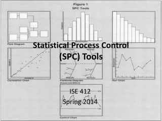
First Steps in Statistical Process Control (SPC) • Measure characteristics of goods or services that are important to customers • Make a control chart for each characteristic • The chart is used to determine whether the process is in control
Types of Measures (1)Variable Measures • Continuous random variables • Measure does not have to be a whole number. • Examples: time, weight, miles per gallon, length, diameter
Types of Measures (2)Attribute Measures • Discrete random variables – finite number of possibilities • Also called categorical variables • The measure may depend on perception or judgment. • Different types of control charts are used for variable and attribute measures
Examples of Attribute Measures • Good/bad evaluations • Good or defective • Correct or incorrect • Number of defects per unit • Number of scratches on a table • Opinion surveys of quality • Customer satisfaction surveys • Teacher evaluations
SPC for VariablesThe Normal Distribution = the population mean • = the standard deviation for the population 99.74% of the area under the normal curve is between - 3 and + 3
SPC for Variables The Central Limit Theorem • Samples are taken from a distribution with mean and standard deviation . k = the number of samples n = the number of units in each sample • The sample means are normally distributed with mean and standard deviation when k is large.
Control Limits for the Sample Mean when and are known • x is a variable, and samples of size n are taken from the population containing x. Given: = 10, = 1, n = 4 Then A 99.7% confidence interval for is
Control Limits for the Sample Mean when and are known (2) The lower control limit for is
Control Limits for the Sample Mean when and are known (3) The upper control limit for is
Control Limits for the Sample Mean when and are unknown • If the process is new or has been changed recently, we do not know and • Example 6.1, page 180 • Given: 25 samples, 4 units in each sample • and are not given • k = 25, n = 4
Control Limits for the Sample Mean when and are unknown (2) • Compute the mean for each sample. For example, • Compute
Control Limits for the Sample Mean when and are unknown (3) • For the ith sample, the sample range is Ri =(largest value in sample i ) - (smallest value in sample i ) • Compute Ri for every sample. For example, R1 = 16.02 – 15.83 = 0.19
Control Limits for the Sample Mean when and are unknown (4) • Compute , the average range • We will approximate by , where A2is a number that depends on the sample size n. We get A2from Table 6.1, page 182
Factor for x-Chart Factors for R-Chart Sample Size (n) A2 D3 D4 2 1.88 0.00 3.27 3 1.02 0.00 2.57 4 0.73 0.00 2.28 5 0.58 0.00 2.11 6 0.48 0.00 2.00 7 0.42 0.08 1.92 8 0.37 0.14 1.86 9 0.34 0.18 1.82 10 0.31 0.22 1.78 11 0.29 0.26 1.74 12 0.27 0.28 1.72 13 0.25 0.31 1.69 14 0.24 0.33 1.67 15 0.22 0.35 1.65 Control Limits for the Sample Mean when and are unknown (5) • n = the number of units in each sample = 4. From Table 6.1, A2= 0.73. The same A2is used for every problem with n = 4.
Control Limits for the Sample Mean when and are unknown (6) • The formula for the lower control limit is • The formula for the upper control limit is
Control Chart for The variation between LCL = 15.74 and UCL = 16.16 is the common cause variation.
Common Cause andSpecial Cause Variation • The range between the LCL and UCL, inclusive, is the common causevariation for the process. When is in this range, the process is in control. • When a process is in control, it is predictable. Output from the process may or may not meet customer requirements. • When is outside control limits, the process is out of control and has special cause variation. The cause of the variation should be identified and eliminated.
Factor for x-Chart Factors for R-Chart Sample Size (n) A2 D3 D4 2 1.88 0.00 3.27 3 1.02 0.00 2.57 4 0.73 0.00 2.28 5 0.58 0.00 2.11 6 0.48 0.00 2.00 7 0.42 0.08 1.92 8 0.37 0.14 1.86 9 0.34 0.18 1.82 10 0.31 0.22 1.78 11 0.29 0.26 1.74 12 0.27 0.28 1.72 13 0.25 0.31 1.69 14 0.24 0.33 1.67 15 0.22 0.35 1.65 Control Limits for R • From the table, get D3 and D4 for n = 4. D3 = 0 D4= 2.28
Control Limits for R (2) • The formula for the lower control limit is • The formula for the upper control limit is
fig_ex06_03 fig_ex06_03
Capable Processes = target = target Statistical Process Control (SPC) SPC for Variables Basic SPC Concepts Types of Measures Variation Attributes Mean charts Range charts Objectives Variables and known First steps , unknown
Capable Transformation Process • Inputs • Facilities • Equipment • Materials • Energy Outputs Goods & Services that meet specifications CapableTransformation Process a specification that meets customer requirements + acapable process (meets specifications) = Satisfied customers and repeat business
Review of Specification Limits • The target for a process is the ideal value • Example: if the amount of beverage in a bottle should be 16 ounces, the target is 16 ounces • Specification limits are the acceptable range of values for a variable • Example: the amount of beverage in a bottle must be at least 15.8 ounces and no more than 16.2 ounces. • The allowable range is 15.8 – 16.2 ounces. • Lower specification limit = 15.8 ounces or LSL = 15.8 ounces • Upper specification limit = 16.2 ounces or USL = 16.2 ounces
Control Limits vs. Specification Limits • Control limits show the actual range of variation within a process • What the process is doing • Specification limits show the acceptable common cause variation that will meet customer requirements. • Specification limits show what the process should do to meet customer requirements
Process is Capable: Control Limits arewithin or on Specification Limits Upper specification limit UCL X LCL Lower specification limit
Process is Not Capable: One or BothControl Limits are Outside Specification Limits UCL Upper specification limit X LCL Lower specification limit
Capability and Conformance Quality • A process is capable if • It is in control and • It consistently produces outputs that meet specifications. • This means that both control limits for the mean must be within the specification limits • A capable process produces outputs that have conformance quality (outputs that meet specifications).
Process Capability Ratio • Use to determine whether the process is capable when = target. • If , the process is capable, • If , the process is not capable.
Example • Given: Boffo Beverages produces 16-ounce bottles of soft drinks. The mean ounces of beverage in Boffo's bottle is 16. The allowable range is 15.8 – 16.2. The standard deviation is 0.06. Find and determine whether the process is capable.
Example (2) • Given: = 16, = 0.06, target = 16 LSL = 15.8, USL = 16.2 The process is capable.
Process Capability Index Cpk • If Cpk > 1, the process is capable. • If Cpk < 1, the process is not capable. • We must use Cpk when does not equal the target.
CpkExample • Given: Boffo Beverages produces 16-ounce bottles of soft drinks. The mean ounces of beverage in Boffo's bottle is 15.9. The allowable range is 15.8 – 16.2. The standard deviation is 0.06. Find and determine whether the process is capable.
CpkExample (2) • Given: = 15.9, = 0.06, target = 16 LSL = 15.8, USL = 16.2 Cpk < 1. Process is not capable.
Capable Processes = target = target Statistical Process Control (SPC) SPC for Variables Basic SPC Concepts Types of Measures Variation Attributes Mean charts Range charts Objectives Variables and known First steps , unknown