Download
1 / 53
530 likes | 654 Vues
Stellar Properties from Red Giants to White Dwarfs. Topics. Distances The Solar Neighborhood Naming the Stars Luminosity and Apparent Brightness More on the Magnitude Scale Stellar Temperatures Stellar Sizes Estimating Stellar Radii The Hertzsprung–Russell Diagram

E N D
Stellar Properties from Red Giants to White Dwarfs
Topics Distances The Solar Neighborhood Naming the Stars Luminosity and Apparent Brightness More on the Magnitude Scale Stellar Temperatures Stellar Sizes Estimating Stellar Radii The Hertzsprung–Russell Diagram The Hipparcos Mission
Topics, cont. Extending the Cosmic Distance Scale Stellar Masses Mass and Other Stellar Properties
Measuring Distances to the Stars Which of these stars is closest to the Sun? Which of these stars is the brightest? Which of these stars has the largest diameter? Which of these stars has the lowest temperature?
Measuring Distances to the Stars A light year is the distance light travels in one year. c = 186,000 mi/s or 300,000 km/s 1ly = 6 trillion miles 1ly = 10 trillion km A light year cannot be measured directly. It is derived, based on measurements of the speed light.
Measuring Distances to the Stars Stellar distances can be measured using parallax: January July
THE PARSEC One parsec is the distance of a star that has a parallax angle of one arc second. D = 1/p, where D = distance in parsec p = parallax in arcseconds Measuring Distances to the Stars
The Solar Neighborhood Nearest star to the Sun: Proxima Centauri which is a member of a 3-star system: Alpha Centauri complex Model of distances: Sun is a marble, Earth is a grain of sand orbiting 1 m away Nearest star is another marble 270 km away Solar system extends about 50 m from Sun; rest of distance to nearest star is basically empty
The Solar Neighborhood Next nearest neighbor: Barnard’s Star Barnard’s Star has the largest proper motion of any – proper motion is the actual shift of the star in the sky, after correcting for parallax. These pictures were taken 22 years apart:
The Solar Neighborhood Actual motion of the Alpha Centauri complex:
The Solar Neighborhood The 30 closest stars to the Sun:
The Solar Neighborhood Naming stars: Brightest stars were known to, and named by, the ancients (Procyon) In 1604, stars within a constellation were ranked in order of brightness, and labeled with Greek letters (Alpha Centauri) In the early 18th century, stars were numbered from west to east in a constellation (61 Cygni)
The Solar Neighborhood As more and more stars were discovered, different naming schemes were developed (G51-15, Lacaille 8760, S 2398) Now, new stars are simply labeled by their celestial coordinates You cannot buy a star and have it named after someone. While these names are registered they are not recognized by the IAU.
Apparent Magnitude • Hipparchus made 1st star catalog in 120 BC. • Divided stars into brightness categories. • 1st mag brightest stars in the sky • 5th mag faintest stars visible to unaided eye.
Magnitude Scale • m=-2.5log(I) • 2nd mag is 2.5x fainter than 1st mag. • 3rd mag is 2.5x fainter than 2nd mag. • 2.5x2.5x2.5x2.5x2.5~100 • So a 5th mag star is about 100x fainter than a 1st mag star.
Apparent Magnitude Scale Apparent luminosity is measured using a magnitude scale, which is related to our perception. It is a logarithmic scale; a change of 5 in magnitude corresponds to a change of a factor of 100 in apparent brightness. It is also inverted – larger magnitudes are dimmer.
Apparent Magnitude Stellar brightness depends on the star’s actual brightness and on its distance. Inverse Square Law Double distance intensity drops by 22. Triple distance intensity drops by 32.
Luminosity and Apparent Brightness Therefore, two stars that appear equally bright might be a closer, dimmer star and a farther, brighter one:
Luminosity and Apparent Brightness Luminosity, or absolute brightness, is a measure of the total power radiated by a star. Apparent brightness is how bright a star appears when viewed from Earth; it depends on the absolute brightness but also on the distance of the star:
Luminosity and Apparent Brightness If we know a star’s apparent magnitude and its distance from us, we can calculate its absolute (actual) luminosity. Absolute magnitude is the brightness stars would appear to be if they were all place at a standard distance of 10 pc. Therefore, absolute magnitude is an actual comparison of stellar luminosity, or brightness.
Stellar Temperatures The color of a star is indicative of its temperature: Red stars are relatively cool, while blue ones are hotter. When I get in my car I turn the heater on to blue and the AC to red.
Stellar Temperatures The radiation from stars is blackbody radiation; as the blackbody curve is not symmetric, observations at two wavelengths are enough to define the temperature: V mag (visual or yellow) B mag (blue) B-V = color index Range = -0.4<B-V<+1.8 blue to red color
Anne Jump Cannon • 1863-1941 • Used objective prism plates to classify star spectra. • A, B … • A class had strongest H lines. • Later her classifications were reorganized by temperature from hottest to coolest. http://www.astrosociety.org/education/resources/womenast_bib03.html
Stellar Temperatures Stellar spectra are much more informative than the blackbody curves. There are seven general categories of stellar spectra, corresponding to different temperatures. From highest to lowest, those categories are: O B A F G K M
Stellar Temperatures Here are their spectra:
Stellar Temperatures Characteristics of the spectral classifications:
Stellar Sizes A few very large, very close stars can be imaged directly using speckle interferometry; this is Betelgeuse:
Stellar Sizes For the vast majority of stars that cannot be imaged directly, size must be calculated knowing the luminosity and temperature: L a R2xT4 Giant stars have radii between 10 and 100 times the Sun’s. Dwarf stars have radii equal to, or less than, the Sun’s. Supergiant stars have radii more than 100 times the Sun’s.
Stellar Sizes Stellar radii vary widely: If L is large and T is small then R is huge because L a R2xT4
Betelgeuse • Spectral class = M2 • Cool red star (3000K) • Very bright star (M = -5.1) • It must be huge! • ~ 1 au in radius • Distance modulus = m-M m = +0.45 m-M = 0.45-(-5.1) = 5.55 It is 5.55 mag away.
The Hertzsprung–Russell Diagram The H–R diagram plots stellar luminosity against surface temperature. This is an H–R diagram of a few prominent stars:
The Hertzsprung–Russell Diagram Once many stars are plotted on an H–R diagram, a pattern begins to form: These are the 80 closest stars to us; note the dashed lines of constant radius. The darkened curve is called the main sequence, as this is position where most stars are plotted. Also indicated is the white dwarf region; these stars are hot but not very luminous, as they are quite small.
The Hertzsprung–Russell Diagram An H–R diagram of the 100 brightest stars looks quite different: These stars are all more luminous than the Sun. Two new categories appear here – the red giants and the blue giants. Clearly, the brightest stars in the sky appear bright because of their enormous luminosities, not their proximity.
The Hertzsprung–Russell Diagram This is an H–R plot of about 20,000 stars. The main sequence is clear, as is the red giant region. About 90% of stars lie on the main sequence; 9% are red giants and 1% are white dwarfs.
Extending the Cosmic Distance Scale • Spectroscopic parallax: has nothing to do with parallax, but does use spectroscopy in finding the distance to a star • Measure the star’s apparent magnitude and spectral class • Use spectral class to estimate luminosity • Apply inverse-square law to find distance
Extending the Cosmic Distance Scale Spectroscopic parallax can extend the cosmic distance scale to several thousand parsecs:
Recall that the spectroscopic sequence is O, B, A, F, G, K, M from hottest to coolest. You use the method of spectroscopic parallax to determine the distance to an F2 star as 43 pc. You later discover that the star has been misclassified and is actually a type G7. The distance to the star must therefore be • Less than 43 pc. • Greater than 43 pc. • The distance is not related to spectral type.
Extending the Cosmic Distance Scale The spectroscopic parallax calculation can be misleading if the star is not on the main sequence. The width of spectral lines can be used to define luminosity classes:
You forgot that the star Betelgeuse is a red giant and apply the method of spectroscopic parallax to determine its distance. How does this affect your distance estimate? • Betelgeuse is closer than your estimate. • Betelgeuse is farther than your estimate. • The distance estimate is not affected by this mistake.
Extending the Cosmic Distance Scale In this way, giants and supergiants can be distinguished from main-sequence stars.
Weighing the Stars Astronomers cannot bring a star into a laboratory and place it on a scale. So, how do astronomers determine the mass of a star?
Binary Stars Recall Kepler’s 3rd Law, P2 = a3. Newton’s revision, P2(M1+M2) = a3. Rearranging terms M1+M2 = a3/P2. The only way to estimate the masses of stars is to observe two stars orbiting a common center of mass.
Binary Stars • Visual • Spectroscopic • Eclipsing
Visual Binaries Determination of stellar masses: Many stars are in binary pairs; measurement of their orbital motion allows determination of the masses of the stars. Visual binaries can be measured directly; this is Kruger 60:
Spectroscopic Binaries Spectroscopic binaries can be measured using their Doppler shifts:
Eclipsing Binaries Finally, eclipsing binaries can be measured using the changes in luminosity:
Mass and Other Stellar Properties Mass is the main determinant of where a star will be on the main sequence:
Mass and Other Stellar Properties Mass is also correlated with radius, and very strongly correlated with luminosity:
Mass and Other Stellar Properties Mass is also related to stellar lifetime: Using the mass–luminosity relationship:
Mass and Other Stellar Properties So the most massive stars have the shortest lifetimes – they have a lot of fuel but burn it at a very rapid pace. On the other hand, small red dwarfs burn their fuel extremely slowly, and can have lifetimes of a trillion years or more.