Download
1 / 23
230 likes | 252 Vues
Understand why estimating costs is essential for optimizing queries, considering various transformations and join orders in query planning. Learn about different strategies like left-deep join trees for efficient query execution.

E N D
Why estimate costs? • Well, sometimes we don’t need cost estimations to decide applying some heuristic transformation. • E.g. Pushing selections down the tree, can be expected almost certainly to improve the cost of a logical query plan. • However, there are points where estimating the cost both before and after a transformation will allow us to apply a transformation where it appears to reduce cost and avoid the transformation otherwise.
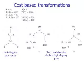
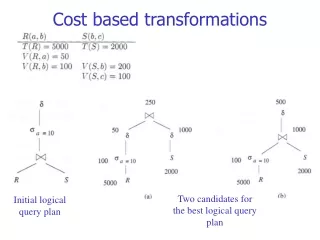
Two candidates for the best logical query plan Initial logical query plan Cost based transformations
Cost based transformations (a) The (estimated) size of a=10(R) is 5000/50 = 100 The (estimated) size of (a=10(R)) is min{1*100, 100/2} = 50 The (estimated) size of (S) is min{200*100, 2000/2} = 1000
Cost based transformations (b) The (estimated) size of a=10(R) is 5000/50 = 100 The (estimated) size of a=10(R)S is 100*2000/200 = 1000
Cost based transformations Adding up the costs of plan (a) and (b), (intermediary relations) we get: • 1150 • 1100 So, the conclusion is that plan (b) is better, i.e. deferring the duplicate elimination to the end is a better plan for this query.
Choosing a join order • Critical problem in cost-based optimization: Selecting an order for the (natural) join of three or more relations. • Cost is the total size of intermediate relations. • We have, of course, many possible join orders • Does it matter which one we pick? • If so, how do we do this?
Basic intuition R(a,b), T(R) = 1000, V(R,b) = 20 S(b,c), T(S) = 2000, V(S,b) = 50, V(S,c) = 100 U(c,d) T(U) = 5000, V(U,c) = 500 (R S) U versus R (S U)? Both plans are estimated to produce the same number of tuples (no coincidence here). However, the first plan is more costly than the second plan because the size of its intermediate relation is bigger than the size of the intermediate relation in the second plan (40K versus 20K) • T(R S) = 1000*2000 / 50 = 40,000 • T((R S)U) = 40000 * 5000 / 500 = 400,000 • T(S U) = 2000*5000 / 500 = 20,000 • T(R (S U)) = 1000*20000 / 50 = 400,000
Joins of two relations (Asymetricity of Joins) • In some join algorithms, the roles played by the two argument relations are different, and the cost of join depends on which relation plays which role. • E.g., the one-pass join reads one relation - preferably the smaller - into main memory. • Left relation (the smaller) is called the build relation. • Right relation, called the probe relation, is read a block at a time and its tuples are matched in main memory with those of the build relation. • Other join algorithms that distinguish between their arguments: • Nested-Loop join, where we assume the left argument is the relation of the outer loop. • Index-join, where we assume the right argument has the index.
title starName=name name StarsIn birthdate LIKE ‘%1960’ MovieStar Not the right order: The smallest relation should be left. Join of two relations • When we have the join of two relations, we need to order the arguments. SELECT movieTitle FROM StarsIn, MovieStar WHERE starName = name AND birthdate LIKE '%1960';
Join of two relations (continued) title starName=name This is the preferred order name StarsIn birthdate LIKE ‘%1960’ MovieStar
Join Trees • There are only two choices for a join tree when there are two relations • Take either of the two relations to be the left argument. • When the join involves more than two relations, the number of possible join trees grows rapidly. E.g. suppose R, S, T, and U, being joined. What are the join trees? • There are 5 possible shapes for the tree. • Each of these trees can have the four relations in any order. So, the total number of tree is 5*4! =5*24 = 120 different trees!!
Ways to join four relations left-deep tree All right children are leaves. righ-deep tree All left children are leaves. bushy tree
Considering Left-Deep Join Trees Good choice because • The number of possible left-deep trees with a given number of leaves is large, but not nearly as large as the number of all trees. • Left-deep trees for joins interact well with common join algorithms - nested-loop joins and one-pass joins in particular. • Query plans based on left-deep trees will tend to be more efficient than the same algorithms used with non-left-deep trees.
Number of plans on Left-Deep Join Trees • For n relations, there is only one left-deep tree shape, to which we may assign the relations in n! ways. • However, the total number of tree shapes T(n)for n relations is given by the recurrence: • T(1)= 1 • T(n)=i=1…n-1T(i)T(n - i) T(1)=1, T(2)=1, T(3)=2, T(4)=5, T(5)=14, and T(6)=42. To get the total number of trees once relations are assigned to the leaves, we multiply T(n)by n!. Thus, for instance, the number of leaf-labeled trees of 6 leaves is 42*6! = 30,240, of which 6!, or 720, are left-deep trees. We may pick any number i between 1 and n - 1 to be the number of leaves in the left subtree of the root, and those leaves may be arranged in any of the T(i)ways that trees with i leaves can be arranged. Similarly, the remaining n-i leaves in the right subtree can be arranged in any of T(n-i)ways.
Left-Deep Trees and One Pass Algo. • A left-deep join tree that is computed by a one-pass algorithm requires main-memory space for at most two of the temporary relations any time. • Left argument is the build relation; i.e., held in main memory. • To compute RS, we need to keep R in main memory, and as we compute RS we need to keep the result in main memory as well. • Thus, we need B(R) + B(RS) buffers. • And so on…
Left-Deep Trees and One Pass Algo. • How much main memory space we need?
Dynamic programming • Often, we use an approach based upon dynamic programming to find the best of the n! possible orders. • Basic logic: Fill in a table of costs, remembering only the minimum information we need to proceed to a conclusion • Suppose we want to join RlR2 …Rn • Construct a table with an entry for each subset of one or more of the n relations. In that table put: • The estimated size of the join of these relations. (We know the formula for this) • The least cost of computing the join of these relations • Basically, this is the size of the intermediate set. • The expression that yields the least cost: the best plan. This expression joins the set of relations in question, with some grouping.
Example R(a,b) V(R,a) = 100 V(R,b) = 200 S(b,c) V(S,b) = 100 V(S,c) = 500 T(c,d) V(T,c) = 20 V(T,d) = 50 U(d,a) V(U,a) = 50 V(U,d) = 1000 Note that the size is simply the size of the relation, while cost = the size of the intermediate set (0 at this stage). Let’s say we start with the basic information below:
Example...cont’d • Based upon the previous results, the table compares options for both left-deep trees (the first four) and bushy trees (the last three) • Option 4 has a cost of 3000. It is a left deep plan and would be chosen by the optimizer
Simple Greedy algorithm • It is possible to do an even simpler form of this technique (if speed is crucial) • Basic logic: BASIS: Start with the pair of relations whose estimated join size is smallest. The join of these relations becomes the current tree. INDUCTION: Find, among all those relations not yet included in the current tree, the relation that, when joined with the current tree, yields the relation of smallest estimated size. The new current tree has the old current tree as its left argument and the selected relation as its right argument. • Note, however, that this is not guaranteed in the general case as dynamic programming is much more powerful.
Example • The basis step is to find the pair of relations that have the smallest join. • This honor goes to the join T U, with a cost of 1000. Thus, T U is the "current tree." • We now consider whether to join R or S into the tree next. • We compare the sizes of (T U)R and (T U)S. • The latter, with a size of 2000 is better than the former, with a size of 10,000. Thus, we pick as the new current tree (T U)S. • Now there is no choice; we must join R at the last step, leaving us with a total cost of 3000, the sum of the sizes of the two intermediate relations.