Download
1 / 19
190 likes | 467 Vues
Outline What is Partitioning Partitioning Example Partitioning Theory Partitioning Algorithms Goal Understand partitioning problem Understand partitioning algorithms. Partitioning. Divide a design into smaller pieces based on a set of constraints Constraints

E N D
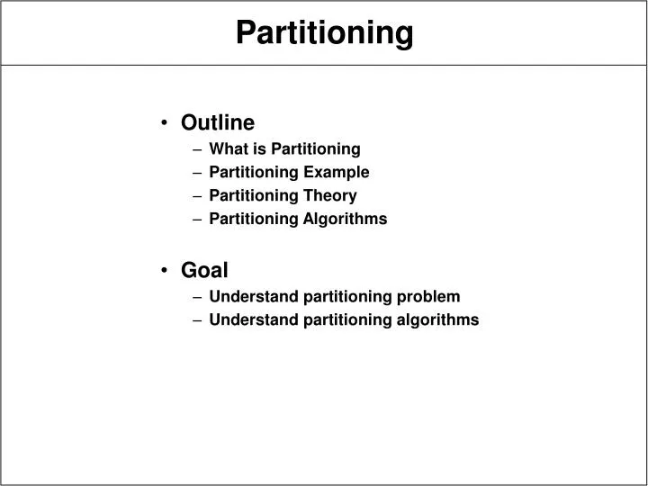
Outline What is Partitioning Partitioning Example Partitioning Theory Partitioning Algorithms Goal Understand partitioning problem Understand partitioning algorithms Partitioning
Divide a design into smaller pieces based on a set of constraints Constraints amount of design in a partition number of nets to/from partition number of partitions allowed balance between partition sizes weight nets crossing partition boundaries Applications divide large design into multiple packages place circuit components on a chip or board What is Partitioning
Constraints 12 transistors per package 7 pins per package few packages as possible nets of equal weight Bounds 30 xistors => >=3 packages 21 terminals => <=3 packages 6 4 6 4 4 6 Partitioning Example 12 xistors 7 pins 12 xistors 5 pins 6 4 6 4 4 6 6 xistors 4 pins 12 xistors 7 pins 8 xistors 5 pins 6 4 10 xistors 6 pins 6 4 etc. 4 6
Partitioning Set Formulation V a set of nodes (components) each node r having area a(r) X a set of nodes (terminals) external to V S = (S1, S2, ..., SN) a set of subsets of V U X Si correspond to nets partition V into disjoint subsets V1, V2,..., Vk such that area of nodes in Vi<= Ai number of sets in S which have nodes external and internal to Viis <= Ti, (pin count) Other formulations graphs - weighted nets, edges connection matrix - eigenvectors Partitioning Theory
Direct seed each module, grow based on constraints Group Migration randomly place components, then move between partitions Metric Allocation goodness metric for each component pair, partition to minimize metric Simulated Annealing shuffle components among partitions to minimize cost function, permit uphill moves to get around local minima Partitioning Algorithms
place a component r from V into each partition Vi pick relatively independent components for each remaining component r in V { for each Vi with area of nodes <= Ai and number of sets in S which have nodes external and internal to Vi <= Ti, compute cost of placing r in Vi place r in lowest-cost Vi } Complexity O(V*k) assumes placement cost computation is O(1) Issues sensitive to initial seeding sensitive to component examination order gets stuck in local minimum Direct Partitioning
D G C F E B A A D Direct Partitioning Example A G E D F B C G, F A E D B C E C A A B E E D D B
1. Partition nodes into groups A and B 2. For every a in A, and every b in B { compute change in terminal counts Da and Db that occur if a and b are swapped.} set queue to empty and i = 1. 3. Select from all pairs (a, b) the pair (ai, bi) that gives most reduction in total terminal count when swapped. add to queue save the improvement in terminal count as gi 4. Remove ai from A and bi from B, recalculate Da and Db. if A and B not empty, i++, go to 3. 5. Find k such that G = sum of g1 to gk is a minimum. swap a1,...ak and b1,...bk. if G < 0 and k > 0, go to 2, else stop. Group Migration
D G C F E B A Group Migration Example Initial Partition, Cutset = 6 Da Db Da Db (A,E) 0 -3 (A,F) -1 0 (A,G) -1 0 (C,E) +1 -3 (C,F) 0 0 (C,G) 0 0 (D,E) -2 -3 (D,F) -2 +1 (D,G) -2 +1 (B,E) +1 -3 (B,F) 0 0 (B,G) 0 0 G Queue 1: (D,E) -5 2: (A,F) +1 (-1,+3) ... C F removed (D,E) B A Final Partition, Cutset = 1 • Minimum G=-5 at k=1 • Swap D and E • Next iteration: • all pairs positive • k=0, quit A D G E B C F
Complexity O(n2) per iteration in worst case for n nodes steps 2, 3 converges in only a few iterations newer versions are O(nlogn) Application to partitioning use bisection divide into two partitions, then split those partitions, etc. partition area is ignored, partitions remain balanced subdivide until partition area is small enough algorithm also called min-cut since it minimizes terminals Group Migration
Approach move one cell at a time between partitions A and B less restrictive than pair moves no longer need to maintain partition size balance use special data structures to minimize cell gain updates only move cells once per pass Complexity prove constant number of updates per cell per pass runtime per pass = O(P) - P pins/terminals vs. O(n2) for group migration small (3-5) number of passes to converge estimate total time is O(PlogP) more pins than nets usually more pins than cells Fiduccia-Mattheyses Algorithm
ni - number of cells on neti si - size (area) of celli smax - largest cell = max(si) S - total size of cells = sum(si) pi - number of pins on celli pmax - most pins on a cell = max(pi) P - total number of pins = sum(pi) C - total number of cells N - total number of nets r - fraction of cell area in partition A CELL - C-entry array, entry is linked list of nets on cell NET - N-entry array, entry is linked list of cells on net Definitions
Cell Gain gi - reduction in cutset by moving celli label each cell with its gain -pi <= gi <= pi -pmax <= gi <= pmax Gain Data Structure BUCKET array of cell gains one per partition O(1) access to cells of a given gain MAXGAIN tracks cells of max gain remove cell once it has moved cells move once per pass gain does not matter after that +2 +1 0 -1 BUCKET +pmax MAX GAIN Cell # Cell # -pmax CELL 1 2 C Cell Gain
Minimize cell gain updates if all cells are updated on each move - O(C2) algorithm only cells that share a net with a moved cell must be updated but big net implies many moves and many updates only cells on critical nets must be updated Critical nets moving a cell would change cutstate cutstate - whether net is cut or not critical only if net has 0 or 1 cells in A or B Critical Nets A=0, B=3 critical A=1, B=2 critical A=2, B=2 not critical
Control size balance between partitions otherwise all cells move to one partition cutset = 0 Balance criterion rS - smax <= |A| <= rS + smax permits some “wiggle room” for cells to move Partition Balance yes no
Initially place cells randomly into A and B Compute cell gains Algorithm for each pass for all cells in A and B of maximum gain whose move would not cause imbalance choose one with best balance result - the base cell if none qualify, quit pass move to opposite partition and lock (remove from BUCKET) unlocked cells are free cells update cell gains and MAXGAIN pointer Repeat passes until no moves occur unlock all cells at beginning of pass Algorithm
F = “from” partition of base cell T = “to” partition of base cell FT(n) = # free T cells of net n FF(n) = # free F cells of net n LT(n) = # locked T cells of net n LF(n) = # locked F cells of net n for each net n on base cell do if LT(n) == 0 if FT(n) == 0 UpdateGains(NET(n)) else if FT(n) == 1 UpdateGains(NET(n)) FF(n)-- LT(n)++ if LF(n) == 0 if FF(n) == 0 UpdateGains(NET(n)) else if FF(n) == 1 UpdateGains(NET(n)) Update Cell Gains
Example Initial partition cutset = 3 si = 1, r = 0.5, 1 <= |A| <= 3 Final partition cutset = 1 +3 +1 +1 -1 L -3 L +1 a b c d b a c d - b, c are highest-gain candidates - choose b, move and lock - recompute gains for a and b - no candidates qualify - quit pass - second pass - no candidates qualify - quit L +1 +1 -1 b a c d -1 -3 -1 +1 - a, c are highest-gain candidates - choose c, move and lock - recompute gains for a, d b a c d
Fast O(PlogP) constant factors are small arrays, pointer access Space Efficient 5 words/net overhead 4 words/cell overhead small constant overhead Suboptimal gets stuck in local minima any one move has negative gain need multiple moves for positive gain Example moving a or b results in -3 or -4 gain moving both a and b results in +1 gain Properties of Algorithm a -3 -3 -4 -4 b