Chapter 7. Filter Design Techniques

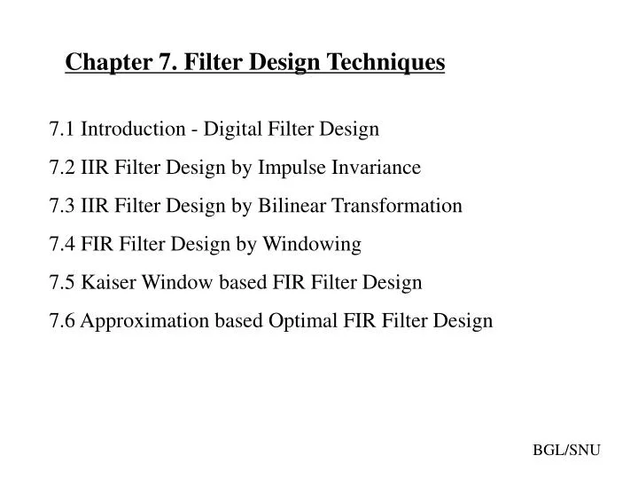
1. Chapter 7. Filter Design Techniques 7.1 Introduction - Digital Filter Design 7.2 IIR Filter Design by Impulse Invariance 7.3 IIR Filter Design by Bilinear Transformation 7.4 FIR Filter Design by Windowing 7.5 Kaiser Window based FIR Filter Design 7.6 Approximation based Optimal FIR Filter Design BGL/SNU

2. 1. Introduction -- Digital Filter Design (1) Frequency selective filters : spectral shapers lowpass highpass bandpass bandstop (2)Filter Design Techniques IIR : - mapping from analog filters - impulse invariance FIR: - windowing - equiripple design BGL/SNU

3. (3)Filter Specification(LPF) In some IIR filter design 1 2 3 1 2 3 BGL/SNU

4. 2. IIR Filter Design by Impulse Invariance (1) Design Concept - Utilize existing analog filter design technique - Convert analog impulse response into digital impulse response h[n] by taking samples - Take Then by fundamental sampling property, we get - If analog filter were bandlimited, Then BGL/SNU

5. (2) Aliasing Problem - But the issue is that the above assumption is not likely, so aliasing is inevitable in reality aliasing • Therefore this design technique is useful only when • designing a narrowband sharp lowpass filters BGL/SNU

6. (3) Parameter Conversion - Let the analog filter has the partial-fraction expansion - After sampling, = = h [ n ] T h (nT ) d c d • Therefore, • pole at in is mapped to Pole at BGL/SNU

7. * Impulse Invariance Filter Design Procedure 1) Given specification in domain. 2) Convert it into specification in domain 3) Design analog filter meeting the specification  4) Convert it into digital filter function H(z) by putting [ 5) Implement it in 2nd order cascade form] BGL/SNU

8. Design Example 1 2 * Choose Td=1 3 BGL/SNU

9. 4 * You plot the pole locations in the z-plans! BGL/SNU

10. 3. IIR Filter Design by Bilinear Transformation (1) Design Concept - s-plane to z-plane conversion • any mapping than maps stable region is s-plane (left half plane) • to stable region in z-plane (inside u.c) ? or bilinear transform! * Td inserted for convention may put to any convenient value for practical use.

11. (2) Properties

12. * IIR Filter Design Procedure Given specification in digital domain Convert it into analog filter specification Design analog filter (Butterworth, Chebyshov, elliptic):H(s) Apply bilinear transform to get H(z) out of H(s) 1 2 3 4 3 2 4 1

13. 3 1 W = 2 | H ( j ) | c + W W 2 N 1 ( / ) c Design Example (Butterworth Filter) Given specification 1 Specification Conversion 2 (Set Td=1) Butterworth filter design

14. Bilinear Transform 4

15. *Comparison of Butterworth, Chebyshev, elliptic filters -Filter equations 1 Butterworth filter B Chebyshev filter (type I) C 1 Chebyshev polynomial

16. *Comparison of Butterworth, Chebyshev, elliptic filters (Cont’d) Chebyshev filter (type II) 1 Elliptic filter E 1 Jacobian elliptic function

17. *Comparison of Butterworth, Chebyshev, elliptic filters: Example -Given specification -Order Butterworth Filter : N=14. ( max flat) Chebyshev Filter : N=8. ( Cheby 1, Cheby 2) Elliptic Filter : N=6 ( equiripple) B C E

18. -Pole-zero plot (analog) B C1 C2 E -Pole-zero plot (digital) B C1 C2 E (14) (8)

19. -Magnitude -Group delay C1 B B E C1 E C2 C2

20. 4. FIR Filter Design by Windowing (1) Design Concept - Given a desired frequency response evaluate - Then, is the desired filter coefficients. However, is infinitely long, so not practical. Therefore, take a finite segment of , or such that the resulting frequency spectrum fall in the given specification. This process of getting out of is called Windowing

21. (2) Rectangular Windowing

22. ) w ) ( j W ( e

24. (3) Design Point w e ( ) : depends on the attenuation of the peak sidelobe of w j W ( e ). But M cannot improve this. (due to Gibb’s phenomena). Therefore, once a specific window is given, is fixed. e ( w ) w D w j : depends on the width of main lobe of W ( e ). This can be improved by increasing M.

25. (4) Commonly Used Windows BGL/SNU

26. BGL/SNU

27. Frequency Spectrum of Windows (a) Rectangular, (b) Bartlett, (c) Hanning, (d) Hamming, (e) Blackman , (M=50) BGL/SNU

28. 5. Kaiser Window based FIR Filter Design (1) Design Concept ( I : 0th order modified Bessel function) 0 • targets at limited duration in time and energy concentration at • low frequency • - compromisable. (choose appropriate ) • Performance comparable to Hamming window ( when ) BGL/SNU

29. Frequency Spectrum of Kaiser Window (a) Window shape, M=20, (b) Frequency spectrum, M=20, (c) beta=6 BGL/SNU

30. (2) Determination of Filter Order ( Kaiser, 1974 ) ① ② ③ BGL/SNU

31. - Design Example : ① ② ③ ④ (Note)

32. BGL/SNU

33. 6. Approximation based Optimal FIR Filter Design (1) Design Concept - Linear phase filters possess the property - More Generally, constant delay filters have the expression BGL/SNU

34. - Approximation error BGL/SNU

35. - Approximation ( Chebyshev) BGL/SNU

36. (2) Type I Lowpass Filter case - desired : - approximation - weighting BGL/SNU

37. - Error function

38. (3) Type II Lowpass Filter case - desired (original) : - approximation BGL/SNU

39. - Weighting (modified) - Desired (modified) - error function BGL/SNU

40. BGL/SNU

41. (4) Alternation Theorem BGL/SNU

42. BGL/SNU

43. BGL/SNU

44. (5) Parks-McClellan Algorithm ① ② ③ ④ BGL/SNU

45. ⑤ Remez Exchange Algorithm (1934) (multiple exchange) ① ② BGL/SNU

46. ③ BGL/SNU

47. ④ ⑤ ⑥ BGL/SNU

48. Selection of new extrema BGL/SNU

49. Initial guess of (L+2) extremal frequencies Remez Exchange Algorithm Calculate the optimum  On extremal set Interpolate through (L+1) Points to obtain Ae(ej) Best approximation Calculate error E() And find local maxima Where | E()|>=  Unchanged Check whether the Extremal points changed Changed More than (L+2) extrema? Yes Retain (L+2) Largest extrema No BGL/SNU

50. Design Examples ① Kaiser, (1974) BGL/SNU