Download
1 / 32
340 likes | 503 Vues
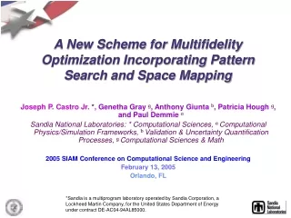
Multifidelity Optimization Via Pattern Search and Space Mapping. Genetha Gray Computational Sciences & Mathematics Research Sandia National Labs, Livermore, CA.

E N D
Multifidelity Optimization Via Pattern Search and Space Mapping Genetha Gray Computational Sciences & Mathematics Research Sandia National Labs, Livermore, CA Sandia is a multiprogram laboratory operated by Sandia Corporation, a Lockheed Martin Company, for the United States Department of Energy’s National Nuclear Security Administration under contract DE-AC04-94AL85000.
Outline • Multifidelity Optimization • APPSPACK • Space Mapping • MFO scheme • Descriptive Example • Groundwater Remediation Example
Finite Element Models of the Same Component High Fidelity 800,000 DOF Low Fidelity 30,000 DOF Multifidelity Optimization (MFO) • The low fidelity model retains many of the properties of the high fidelity model but is simplified in some way • Decreased physical resolution • Decreased FE mesh resolution • Simplified physics • MFO optimizes an inexpensive, low fidelity model while making periodic corrections using the expensive, high fidelity model. • Works well when low-fidelity trends match high-fidelity trends.
Asynchronous Parallel Pattern Search (APPS) • Direct method → no derivatives required • Pattern of search directions drives search and determines new trial points for evaluation • Objective function can be an entirely separate program • Achieves parallelism by assigning function evaluations to different processors • Freely available software under the GNU public license (APPSPACK)
Synchronous Pattern Search Inherently (or embarrassingly) parallel,but processor load should be considered.
Processor Load Balance Considerations • The number of trial points can varyat each iteration. • Cached function values • Search patterns change • Constraints (infeasible trial points are not evaluated) • Evaluation times can vary for each trial point. • Different processor characteristics • Effect of input on function • Function evaluation faults • MFO: different function models with different evaluation times!!
Workers Waiting APPSPACK Example
Workers b c d e Waiting APPSPACK Example
Workers c d Waiting APPSPACK Example
Workers f c d g Waiting APPSPACK Example
Workers c d Waiting APPSPACK Example
Workers h c d i Waiting APPSPACK Example j,k
Workers i Waiting APPSPACK Example
Workers l m n i Waiting APPSPACK Example o
Workers i Waiting APPSPACK Example
Workers p q r i Waiting APPSPACK Example s
Workers Waiting APPSPACK Example Note: Cannot Prune on Unsuccessful Iteration s
Workers s u t v Waiting APPSPACK Example
xH xH high-fi model mapped low-fi model xL=P(xH) RL(P(xH))~RH(xH) such that RL(P(xH)) RH(xH) We’re using the mapping Space Mapping*: A Conduit Between the Low and High Fidelity Model Design Spaces x – design variables R - response P - mapping xL ? P(xH) low-fi model RL(xL) • Space mapping* is a technique that maps the design space of a low fidelity model to the design space of high fidelity model such that both models result in approximately the same response. • The parameters within xH need not match the parameters within xL *Developed by John Bandler, et. al.
Oracle • An oracle predicts points at which a decrease in the objective function might be observed. • Analytically, an oracle can choose points by any finite process. • Oracle points are used in addition to the points defined by the search pattern. • The MFO scheme employs an oracle framework to do a space mapping so that APPSPACK convergence is not adversely affected. • Future work may include investigating any convergence improvement.
Oracle The MFO Scheme: Combining APPSPACK and Space Mapping Outer Loop Inner Loop multiple xH,f(xH) Space Mapping Via Nonlinear Least Squares Calculation High Fidelity Mode Optimization via APPSPACK a,b,g Low Fidelity Model Optimization a (xH) b + g xHtrial
MFO Algorithm • Start the Outer Loop (APPSPACK) • Evaluate N high fidelity response points • Produce xH, fH(xH) pairs • Start the Inner Loop • Take data pairs from APPSPACK • Run LS optimization • At each iteration, evaluate N low fidelity responses • At conclusion, obtain a, b, g for space map a(xH)b + g • Optimize low fidelity model within space mapped high fidelity space. In other words, minimize fL(a(xH)b + g) with respect to xH to obtain xH*. • Return xH* to APPSPACK to determine if a new best point has been found.
A Simple Example View of Unmapped Low Fidelity Design Space View of High Fidelity Design Space
When the # response points is 8, there are two calls to inner loop. Approximate Inner Loop Call Locations within Hi-Fi Model (-0.8,-1.2) 2 1 (-0.76,2.0) 1 • The numbered white boxes show approximately where the inner loop was called • The point in red brackets is where APPSPACK is before the inner loop call • The point in green was found by the inner loop (-0.56,1.6) 2 (-0.61,1.25)
Groundwater Remediation via Optimization • Optimization techniques can aid the design process to result in lower clean up costs. • Use Hydraulic Capture (HC) models to alter the groundwater flow direction and control plume migration • Transport Based Concentration Control (TBCC) • Computationally expensive • Well defined plume boundary → MFO high fidelity model • Flow Based Hydraulic Control (FBHC) • Orders of magnitude faster • Constraints require calibration → MFO low fidelity model
Objective Function J(u) = installation costs + operation costs Evaluation requires results of a simulation Design Variables Number of wells Well pumping rates Well locations Constraints Well capacity Net pumping rate Don’t flood or dry out land No useless wells Implementation Derivatives are unavailable Simulators MODFLOW: used for flow equation (USGS) MT3D: used for transport equation (EPA) Optimization
MFO Numerical Test • Test the MFO method on the HC problem included in the community problems set. (Mayer, Kelley, Miller) • The FBHC formulation has been shown to be sufficient for this simple domain. (Fowler, Kelley, Kees, Miller) • Other approaches are needed for heterogeneous more realistic domains. (Ahlfeld, Page, Pinder)
MFO Results Initial cost: $78,586 MODFLOW (mf2k): ~2 seconds mt3d: ~50 seconds
MFO development team (Sandia) Joe Castro (PI), Electrical & Microsystem Modeling, NM Tony Giunta, Validation & Uncertainty Quantification Processes, NM Patty Hough, CSMR, CA Groundwater Application Katie Fowler, Clarkson University Questions?? Genetha Gray gagray@sandia.gov Acknowledgements • Software • APPSPACK: software.sandia.gov/appspack/version4.0/index.html • DAKOTA: http://endo.sandia.gov/DAKOTA