Download
1 / 57
590 likes | 782 Vues
Section 4: Synoptic Easterly Waves. Section 4: Synoptic Easterly Waves. 4.1 Introduction 4.2 The Mean State over West Africa 4.3 Observations of African Easterly Waves 4.4 Theory 4.5 Modeling 4.6 Hot Topics: 4.6.1 Genesis 4.6.2 Scale Interactions

E N D
Section 4: Synoptic Easterly Waves 4.1 Introduction 4.2 The Mean State over West Africa 4.3 Observations of African Easterly Waves 4.4 Theory 4.5 Modeling 4.6 Hot Topics: 4.6.1 Genesis 4.6.2 Scale Interactions 4.6.3 Relationship to Tropical Cyclogenesis 4.7 Easterly Waves in other Tropical Regions 4.8 Final Comments
4.1 Introduction • Westward moving synoptic waves characterize the whole tropics • They are tropospheric waves, that modulate the rainfall and move at about 8m/s and have wavelengths of 2000-4000km.
4.1 Introduction • The environments that they are embedded in varies around the tropics, and so details of the wave characteristics also vary.
SAL AEWs TC MCSs 4.1 Introduction The emphasis here will be on African Easterly Waves (AEWs) Have a strong influence on daily rainfall patterns over Africa and tropical Atlantic Most Atlantic Tropical Cyclones are generated in association with AEWs
4.2 The Mean State over West Africa Burpee, R.W. 1972 The origin and structure of easterly waves in the lower troposphere of North Africa, J. Atmos. Sci. 29, 77-90 Notable Features: 600mb African Easterly Jet (AEJ) Upper-level Tropical Easterly Jet (TEJ) Low-level Monsoonal Westerlies Low-level Easterlies north of the AEJ Upper-level Westerly Jet to the North
4.2 The Mean State over West Africa Reed, R.J., Norquist, D.C. and Recker, E.E., The structure and properties of African wave disturbances as observed during Phase III of GATE, Mon. Wea. Rev. 105, 317-333 (1977).
PV View of the African Easterly Jet Discussion Consider the meridional contrasts in convection (next slide) and the diabatic source/sink term in the PV-equation.
Schematic of African Easterly Jet AEJ 50oC 90oC θ θe θe θ 20oC 60oC
4.2 The Mean State over West Africa Thorncroft and Blackburn 1999
Zonal Variations in the Mean State Mean 700hPa U wind, 16th July – 15th August 2000 Berry and Thorncroft 2005
Zonal Variations in the Mean State 925hPa q 315K PV • PV ‘strip’ present on the cyclonic shear side of AEJ. • Strong baroclinic zone 10o-20oN 925hPa qe • High qe strip exists near 15oN
4.3 Observations of African Easterly Waves Carlson, T.N., 1969a: Synoptic histories of three African disturbances that developed into Atlantic hurricanes. Mon. Wea. Rev., 97, 256-276. Carlson, T.N., 1969b: Some remarks on African disturbances and their progress over the tropical Atlantic. Mon. Wea. Rev., 97, 716-726. Burpee, R.W., 1970: The origin and structure of easterly waves in the lower troposphere of North Africa, J. Atmos. Sci. 29, 77-90. Reed, R.J., Norquist, D.C. and Recker, E.E., 1977: The structure and properties of African wave disturbances as observed during Phase III of GATE, Mon. Wea. Rev. 105, 317-333 Thorncroft, C.D. and Hodges: 2001 K.I., African easterly wave variability and its relationship to tropical cyclone activity, J. Clim.14, 1166-1179 (2001). Kiladis, G., C. Thorncroft, and N. Hall, 2006: Three-Dimensional Structure and Dynamics of African easterly waves: part I: Observations, J. Atmos. Sci., 63, 2212-2230. Mekonnen, A., C. Thorncroft, and A. Aiyyer, 2006: On the significance of African easterly waves on convection, J. Climate, 19, 5405-5421. Berry, G., Thorncroft, C.D. and Hewson, T. 2006 African easterly waves in 2004 – Analysis using objective techniques Mon. Wea. Rev., 133, 752-766
4.3 Observations of African Easterly Waves Carlson 1969ab Carried out case studies of several AEWs Peak amplitudes at 600-700mb and at surface Eastward tilt with height from the surface to the level of the AEJ Two cyclonic centers at low-levels Synoptic variations in cloud cover Peak of cloudiness close to AEW trough
4.3 Observations of African Easterly Waves Burpee (1970) Eastward tilt beneath the AEJ – Westward tilt above the AEJ Northerlies dry and warm Southerlies wet and cold
4.3 Observations of African Easterly Waves Reed et al, 1977 Composite AEW structures from phase III of GATE (after Reed et al, 1977). (a) and (b) are relative vorticity at the surface and 700hPa respectively with a contour interval of 10-5s-1. (c) and (d) show percentage cover by convective cloud and average precipitation rate (mm day-1) respectively. Category 4 is location of 700hPa trough and the “0” latitude is 11oN over land and 12oN over ocean.
4.3 Observations of African Easterly Waves Thorncroft and Hodges (2001)
Three Dimensional Structure of Easterly Wave Disturbances over Africa and the Tropical North Atlantic George N. Kiladis 1 Chris D. Thorncroft 2 Nick M. J. Hall 3 1 NOAA Aeronomy Laboratory, Boulder, CO 2 Dept. of Atmospheric Sciences, SUNY, Albany, NY 3 LTHE, Grenoble, France
Space-Time Spectrum of JJA Antisymmetric OLR, 15S-15N Wheeler and Kiladis, 1999
Regression Model Simple Linear Model: A separate linear relationship between a predictor at a grid point and a parameter at every other grid point is obtained: y = ax + b where: x= predictor (TD-filtered OLR at 10N, 10W) y= predictand (u or v wind at any grid point) Maps or cross sections at lag can then be constructed to show the evolution of the dynamical fields versus the predictor
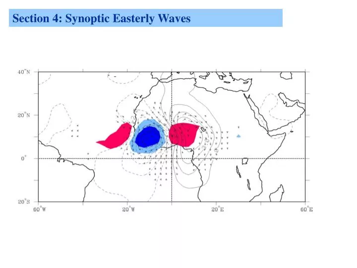
OLR and 850 hPa Flow Regressed against TD-filtered OLR (scaled -20 W m2) at 10N, 10W for June-September 1979-1993 Day 0 Streamfunction (contours 1 X 10⁵ m2 s-1) Wind (vectors, largest around 2 ms-1) OLR (shading starts at +/- 6 W s-2), negative blue
OLR and 850 hPa Flow Regressed against TD-filtered OLR (scaled -20 W m2) at 10N, 10W for June-September 1979-1993 Day-4 Streamfunction (contours 1 X 10⁵ m2 s-1) Wind (vectors, largest around 2 ms-1) OLR (shading starts at +/- 6 W s-2), negative blue
OLR and 850 hPa Flow Regressed against TD-filtered OLR (scaled -20 W m2) at 10N, 10W for June-September 1979-1993 Day-3 Streamfunction (contours 1 X 10⁵ m2 s-1) Wind (vectors, largest around 2 ms-1) OLR (shading starts at +/- 6 W s-2), negative blue
OLR and 850 hPa Flow Regressed against TD-filtered OLR (scaled -20 W m2) at 10N, 10W for June-September 1979-1993 Day-2 Streamfunction (contours 1 X 10⁵ m2 s-1) Wind (vectors, largest around 2 ms-1) OLR (shading starts at +/- 6 W s-2), negative blue
OLR and 850 hPa Flow Regressed against TD-filtered OLR (scaled -20 W m2) at 10N, 10W for June-September 1979-1993 Day-1 Streamfunction (contours 1 X 10⁵ m2 s-1) Wind (vectors, largest around 2 ms-1) OLR (shading starts at +/- 6 W s-2), negative blue
OLR and 850 hPa Flow Regressed against TD-filtered OLR (scaled -20 W m2) at 10N, 10W for June-September 1979-1993 Day 0 Streamfunction (contours 1 X 10⁵ m2 s-1) Wind (vectors, largest around 2 ms-1) OLR (shading starts at +/- 6 W s-2), negative blue
OLR and 850 hPa Flow Regressed against TD-filtered OLR (scaled -20 W m2) at 10N, 10W for June-September 1979-1993 Day+1 Streamfunction (contours 1 X 10⁵ m2 s-1) Wind (vectors, largest around 2 ms-1) OLR (shading starts at +/- 6 W s-2), negative blue
OLR and 850 hPa Flow Regressed against TD-filtered OLR (scaled -20 W m2) at 10N, 10W for June-September 1979-1993 Day+2 Streamfunction (contours 1 X 10⁵ m2 s-1) Wind (vectors, largest around 2 ms-1) OLR (shading starts at +/- 6 W s-2), negative blue
OLR and 850 hPa Flow Regressed against TD-filtered OLR (scaled -20 W m2) at 10N, 10W for June-September 1979-1993 Day+3 Streamfunction (contours 1 X 10⁵ m2 s-1) Wind (vectors, largest around 2 ms-1) OLR (shading starts at +/- 6 W s-2), negative blue
OLR and 850 hPa Flow Regressed against TD-filtered OLR (scaled -20 W m2) at 10N, 10W for June-September 1979-1993 Day+4 Streamfunction (contours 1 X 10⁵ m2 s-1) Wind (vectors, largest around 2 ms-1) OLR (shading starts at +/- 6 W s-2), negative blue
OLR and 850 hPa Flow Regressed against TD-filtered OLR (scaled -20 W m2) at 10N, 10W for June-September 1979-1993 Day+5 Streamfunction (contours 1 X 10⁵ m2 s-1) Wind (vectors, largest around 2 ms-1) OLR (shading starts at +/- 6 W s-2), negative blue
4.3 Observations of African Easterly Waves All the previous slides refer to composite AEW structures They say little about the significance of AEWs on convection and They say little about how these structures might be manifested on a weather map or how they may vary in space and time. The next slides address the significance issue from Mekonnen et al (2006) This will be followed by some maps of individual AEWs (Berry et al 2007).
TB variance (in K2) E. Atlantic E. Atlantic (5-10N, 40W-20W) Land (10-15N, 15W-40E) W. Africa Central Africa Significant time scales: 2-6 days & at 1 day. Peak periods change from west to east E. Africa Shaded region: power > red noise
TB variance (in K2) E. Atlantic W. Africa Central Africa Significant time scales: 2-6 days & at 1 day. Peak periods change from west to east E. Africa Shaded region: power > red noise
TB variance (in K2) E. Atlantic W. Africa Central Africa Significant time scales: 2-6 days & at 1 day. Peak periods change from west to east E. Africa Shaded region: power > red noise
TB variance (in K2) E. Atlantic W. Africa Central Africa Significant time scales: 2-6 days & at 1 day. Peak periods change from west to east E. Africa Shaded region: power > red noise
TB variance (in K2) E. Atlantic W. Africa Central Africa Significant time scales: 2-6 days & at 1 day. Peak periods change from west to east E. Africa Shaded region: power > red noise
2-6d TB variance (shaded >140K2) west-east variance is nearly the same Variance explained by 2-6d TB (shaded > 20%) 2-6d contribution: 25-35% over land, 35-40% over ocean
Comparison with dynamic measures ….. 2-6d 700-hPa variance Land: maximum along 10N, south of the AEJ, near peak convective region. Ocean: near 20N (shaded >5m2s-2) 2-6d 850-hPa variance Land: maximum to the north of AEJ, and over the coast, near peak convective region Ocean: within ITCZ Variance in the west are higher than in the east!
Diagnostics for highlighting multi-scale aspects of AEWs 315K Potential Vorticity (Coloured contours every 0.1PVU greater than 0.1 PVU) with 700hPa trough lines and easterly jet axes from the GFS analysis (1 degree resolution), overlaid on METEOSAT-7 IR imagery. Berry et al 2006
315K Potential Vorticity (Coloured contours every 0.1PVU greater than 0.1 PVU) with 700hPa trough lines and easterly jet axes from the GFS analysis (1 degree resolution), overlaid on METEOSAT-7 IR imagery.
315K Potential Vorticity (Coloured contours every 0.1PVU greater than 0.1 PVU) with 700hPa trough lines and easterly jet axes from the GFS analysis (1 degree resolution), overlaid on METEOSAT-7 IR imagery.
315K Potential Vorticity (Coloured contours every 0.1PVU greater than 0.1 PVU) with 700hPa trough lines and easterly jet axes from the GFS analysis (1 degree resolution), overlaid on METEOSAT-7 IR imagery.
315K Potential Vorticity (Coloured contours every 0.1PVU greater than 0.1 PVU) with 700hPa trough lines and easterly jet axes from the GFS analysis (1 degree resolution), overlaid on METEOSAT-7 IR imagery.
315K Potential Vorticity (Coloured contours every 0.1PVU greater than 0.1 PVU) with 700hPa trough lines and easterly jet axes from the GFS analysis (1 degree resolution), overlaid on METEOSAT-7 IR imagery.
315K Potential Vorticity (Coloured contours every 0.1PVU greater than 0.1 PVU) with 700hPa trough lines and easterly jet axes from the GFS analysis (1 degree resolution), overlaid on METEOSAT-7 IR imagery.
315K Potential Vorticity (Coloured contours every 0.1PVU greater than 0.1 PVU) with 700hPa trough lines and easterly jet axes from the GFS analysis (1 degree resolution), overlaid on METEOSAT-7 IR imagery.
315K Potential Vorticity (Coloured contours every 0.1PVU greater than 0.1 PVU) with 700hPa trough lines and easterly jet axes from the GFS analysis (1 degree resolution), overlaid on METEOSAT-7 IR imagery.
315K Potential Vorticity (Coloured contours every 0.1PVU greater than 0.1 PVU) with 700hPa trough lines and easterly jet axes from the GFS analysis (1 degree resolution), overlaid on METEOSAT-7 IR imagery.
315K Potential Vorticity (Coloured contours every 0.1PVU greater than 0.1 PVU) with 700hPa trough lines and easterly jet axes from the GFS analysis (1 degree resolution), overlaid on METEOSAT-7 IR imagery.