Download
1 / 59
600 likes | 795 Vues
Measurement and Evaluation of Cloud Free Line of Sight with Digital Whole Sky Imagers. BACIMO ‘05. Janet E. Shields, Art R. Burden, Richard W. Johnson, Monette E. Karr, and Justin G. Baker. Overview. Review of Lund CFLOS Data Overview of the Day/Night WSI

E N D
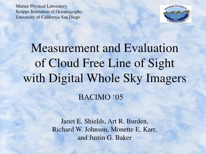
Measurement and Evaluationof Cloud Free Line of Sightwith Digital Whole Sky Imagers BACIMO ‘05 Janet E. Shields, Art R. Burden, Richard W. Johnson, Monette E. Karr, and Justin G. Baker
Overview • Review of Lund CFLOS Data • Overview of the Day/Night WSI • CFLOS Results, Interpretation, and Application • Persistence Results and Application
CFLOS Applications • Detection of objects through the atmosphere by humans and other detectors • Laser propagation including HEL applications and communication • Modeling of the cloud field for cloud simulators, scene simulators and other applications
Characteristics of CFLOS • Probability of Cloud Free Line of Sight (PCFLOS) in a given direction depends on Zenith angle and cloud fraction • Cloud fraction climatologies are used to apply results to multiple sites • Many current applications use the Lund data
Lund Data • Images acquired with a fisheye lens and infrared film • Template was overlaid on images • Visual assessment of CFLOS • Total sky cover from National Weather Service • Hourly data acquired in Columbia, Missouri, over 3 summers during 1966 – 1969, and 3 times per day over 3 years
Goals in using WSI Data • Extract data down to horizon • Extract significantly larger data sample • More images • More angles extracted per image • Use more accurate determination of CFLOS as well as cloud fraction • Potential to extract many sites and seasons, 3 million image sets available so far
Development of WSI Concept • Radiometric scanners and analog fisheye imagers in 60’s, 70’s • First Digital WSI Fielded 1984 • Automated, field-hardened in mid 80’s • 24-hour with night capability in early 90’s • Airborne, NIR, etc. 00’s
1963 WSI 1963 Version
Day WSI Cam Hsg Day WSI Used in late 1980’s Includes digital camera, filter changer, solar occultor, cloud algorithms Data acquisition was Fully automated, System was Environmentally hardened
Day/Night WSI Day/Night WSI System Fielded in Oklahoma, Arctic, Tropics, and other locations This system runs autonomously 24 hours a day
SWIR Airborne Day Vis/NIR WSI Related Systems Modernized D/N WSI
Day/Night Whole Sky Imagers • Ground-based Sky and Cloud Imagery • Daylight, moonlight, and starlight, over 10 decade dynamic range • Full hemisphere, 1/3˚ spatial resolution • Visible and NIR, 4 spectral bands in most systems • Fully automated and autonomous • Environmentally Hardened
Day Image Daytime Image
Moonlight Image Moonlight Image with Cirrus
Milky Way Starlight Image showing Milky Way
Clouds with starlight Starlight Image with clouds
Cloud Decision Algorithms • Algorithm yields Cloud Fraction, cloud decision at each pixel • Opaque clouds are based on fixed spectral signature (red/blue ratio) • Thin clouds are based on perturbations from the clear sky background spectral signature • Night algorithms based on detection of approximately 2000 stars per image
WSI Study • Primarily used Day/Night WSI • Study based on 7000 images from 9 months of data from Oklahoma • Data Evaluated as a function of Cloud Type • Conclusions evaluated using Day WSI data • Day WSI used 95,000 images from 24 months at each of 4 stations
Data Extraction • Images were sorted to remove algorithm artifacts (false cloud at dawn due to red sky) • Solar disk and star positions were carefully analyzed to verify angles in object space for pixels • Data masked to remove obstructions • Data extracted at 5° zenith increments to 80°, then 1° increments; 15° azimuth
Figure 1. Sample output from SubDec_SGP.pro using the cloud decision image collected at 2012 UTC on March 12, 2002. The program superimposes the sampled cloud decision results on the original color-coded cloud decision image for visual comparison.
Data processing vs cloud type • Cloud type was reported hourly by site personnel • Cloud images were evaluated to provide cloud type for images between the hour • Used Lund’s cloud types
Cloud Types • Type 1: Cirroform: Cirrus, Cirrostratus, Cirrocumulus • Type 2: Mid-level: Altucumulus, Altocumulus castellanus, Altostratus • Type 3: Cumuloform (low level convective): Cumulus, Cumulonimbus, Cumulonimbus mammatus, Fractocumulus • Type 4: Stratiform (low level non-convective): Stratus, Nimbostratus, Fractostratus, Stratocumulus
Data Points at each zenith angle as a function of cld fraction and cld type
Probability of Cloud Free Line of Sight (PCFLOS) Opaque and Thin Cloud vs. Zenith Angle and Total Cloud Fraction All Cloud Forms
Probability of Cloud Free Line of Sight (PCFLOS) Opaque Cloud vs. Zenith Angle and Total Cloud Fraction All Cloud Forms
Probability of Cloudy Line of Sight (PCLOS) Is the inverse Of PCFLOS PCLOS PCFLOS
WSI vs. Lund PCFLOS • Lund PCFLOS appears to be too high • PCFLOS should be roughly 1 – Cld fraction • PCFLOS (.9) is near .1 in WSI data, near .3 in Lund data • PCFLOS (.6) is near .4 in WSI data, near .7 in Lund data • Lund data appears to have an inconsistency between CFLOS and cloud cover from visual observers • Impact of the source of the cloud cover statistics should be further investigated
Comparison of WSI PCFLOS and Lund PCFLOS
Near Horizon Behavior • WSI data behave differently than Lund data near the horizon • CFLOS increases toward horizon under broken conditions • CFLOS decreases faster toward horizon under scattered cld • This behavior starts near 50˚ zenith angle, not just in the last few degrees
Comparison of WSI PCFLOS and Lund PCFLOS
Why we believe this Horizon Behavior is real • All 78 images in February data set with 0.8 sky cover were inspected, and horizon clearing is not an artifact of the algorithm • Strong trends even in zenith angle 50° - 80° region (not limited to close to the horizon) • Day WSI behavior is the same as D/N WSI behavior EXCEPT for Opaque clouds at Columbia MO • The behavior is reasonble for contiguous cloud sheets with little vertical development
Day WSI PCFLOS Opaque and Thin White Sands Missile Range 24,000 Images Approx. 9.6 million points
Day WSI PCFLOS Opaque only Columbia, MO 23,100 Images Approx. 9.2 million points Opaque clouds at Columbia behave like Lund; other Day WSI Data shows the more complex horizon behavior seen with the D/N WSI.
WSI PCFLOS vs cloud type Cirroform, High Mid-level (Alto Cu etc) Cumuliform, Low Convective Stratiform, Low Non-convective
PCFLOS Conclusions • WSI data for opaque clouds taken at the same station as the Lund data behave similarly to the Lund data • Other stations commonly show an increase in PCFLOS at the horizon for broken clouds • Similarly, there is a sharper drop in PCFLOS at the horizon for scattered clouds • In addition, Lund CFLOS values appear to be too high, perhaps due to a lack of thin clouds
Applying the CFLOS Results αCs CFLOS Matrix as a function of sky cover (s) and zenith angle () Cloud climatology vector 1 as a function of cloud fraction K1 Resulting CFLOS probability as a function of zenith angle () for climatology 1, using Method A αP1A
CFLOS Matrix Sky Cover (tenths) Zen Ang (deg) 0 1 2 3 4 5 6 7 8 9 10 0 1.00 0.98 0.93 0.83 0.72 0.59 0.37 0.29 0.15 0.07 0.00 10 1.00 0.98 0.92 0.83 0.72 0.59 0.37 0.29 0.15 0.06 0.00 20 1.00 0.98 0.91 0.83 0.72 0.59 0.37 0.29 0.15 0.06 0.00 30 1.00 0.97 0.90 0.82 0.72 0.59 0.38 0.28 0.16 0.05 0.00 40 1.00 0.97 0.90 0.81 0.71 0.59 0.41 0.29 0.17 0.05 0.00 50 1.00 0.96 0.88 0.78 0.69 0.57 0.44 0.30 0.18 0.06 0.00 60 1.00 0.95 0.84 0.74 0.65 0.54 0.43 0.31 0.19 0.07 0.00 70 0.99 0.91 0.78 0.65 0.56 0.46 0.40 0.30 0.20 0.09 0.00 80 0.98 0.85 0.70 0.56 0.47 0.38 0.36 0.28 0.21 0.12 0.01 81 0.98 0.82 0.66 0.52 0.43 0.34 0.34 0.28 0.21 0.14 0.01 82 0.98 0.81 0.64 0.50 0.41 0.32 0.34 0.28 0.22 0.16 0.01 83 0.97 0.80 0.63 0.49 0.40 0.32 0.34 0.29 0.24 0.18 0.01 84 0.96 0.79 0.62 0.48 0.40 0.32 0.35 0.31 0.26 0.21 0.02 85 0.94 0.76 0.61 0.48 0.39 0.33 0.36 0.32 0.28 0.23 0.03 86 0.90 0.73 0.59 0.48 0.40 0.34 0.37 0.35 0.31 0.26 0.03 87 0.86 0.70 0.58 0.48 0.40 0.36 0.39 0.36 0.33 0.28 0.04 88 0.82 0.66 0.56 0.48 0.41 0.37 0.40 0.38 0.35 0.30 0.04
Using Cloud Type • If a matrix of probability of cloud fraction and cloud type is known for a site, Lund’s method B may be used • Method B uses CFLOS as a fn of cloud type, and cloud climatology for cloud type and amount • In the absence of this information, we recommend using cloud type to determine a range of likely results


![[PDF] Free Download Tom Clancy's Line of Sight By Mike Maden](https://cdn4.slideserve.com/7902467/slide1-dt.jpg)