Download
1 / 28
280 likes | 562 Vues
Modeling the Effect of Inducible Plant Defenses on Mobile Herbivore Populations . From “The Effects of Inducible Plant Defenses on Herbivore Populations. 1. Mobile Herbivores in Continuous Time” by Lead Edelstein-Keshet and Mark D. Rausher. Background Information.

E N D
Modeling the Effect of Inducible Plant Defenses on Mobile Herbivore Populations From “The Effects of Inducible Plant Defenses on Herbivore Populations. 1. Mobile Herbivores in Continuous Time” by Lead Edelstein-Keshet and Mark D. Rausher.
Background Information • Inducible Defense - any change in the composition of the foliage caused by consumption and having an adverse affect on the herbivore population. • We are interested in finding out how inducible defenses can change the dynamics of a system.
What are we trying to find out? • Under what circumstances can inducible defenses by themselves regulate populations of herbivores? • Will there be steady-states? • Will they be stable?
How is this different from our other models? • In this model the quality of the resource that limits growth as opposed to the quantity or resource. • Here we model the resource itself as a dynamical variable instead of assuming that it is in a static state.
Assumptions: • Herbivores are mobile and non-selective. An individual herbivore is not constrained to a locale and will have an almost uniform effect on the plants it feeds upon. • Examples: • Snowshoe hares (Reichardt et al. 1984) • Beetles (Karieva 1982) • Ungulates of the African Savannah (Pennycuick 1975) • Various Orthoptera (Gangwere 1961; Otte 1975; Otte and Joern 1977).
More Assumptions • Induced Defenses have a negative impact on herbivore population. • Rate of removal of plants is unaffected by inducement. • Plants develop induced defense after being grazed upon and the levels of induced defense decay with time. • New plants enter the population at a rate proportional to the biomass of plants. • There is a maximum inducible level, qmax.
Dynamic Variables in the Model • q - the level of inducible factor in an individual unit of foliage • t - time • p(q,t) - amount of foliage with inducible factor at level q at time t • Qbar - average value of q in foliage • h(t) - the density of herbivores per unit foliage at time t • H(t) - total herbivore population • P(t) - total amount of foliage • sigma is the rate of removal of vegetation.
The following describe a single unit of vegetation dq/dt = f(q,h) dh/dt = g(q,h) Where f(q,h) reflects the change in plant defense in response to current defense level coupled with current herbivore level and g(q,h) reflects the change in the number of herbivores in response to current level of herbivores and current level of plant defense. Modeling a Single Unit of Vegetation
Modeling Entire Plant Population • So for the entire plant population: • dp/dt = -d(fp)/dq - sigma*p • Note that sigma is a function of herbivore population and total plant population (note that sigma is not dependent on plant defenses since we are considering non-selective herbivores). • Note also that the above is a PDE.
Refining Our Model • Because of mobility and non-selectivity the density of herbivores should be almost uniform over the area of vegetation. • So we can write • dh/dt = h*R(Qbar,h) • Where R is the per capita rate of herbivore increase and h is the current density of the herbivores.
Refining Plant Defense Response • Now we can write f(q,h) = S(h) - a*q • Where S is the rate of induction of defenses and a*q represents the spontaneous decay of plant defense.
Refining the Introduction of New Plants • Birthrate of new plants = f(0,h)*p(0,t) = Bbar*P • We can write this since new plants are assumed to have no defense and enter the population at a rate proportional to total plant population.
Refined General Model • dP/dt = P(Bbar - sigma) • dQbar/dt = S(h) - Qbar*(a + Bbar) • dh/dt = h*R(Qbar,h) • note that the equations modeling herbivore density and average induced defense are independent of total plant population we can solve them without considering total plant population.
Evaluating the Different Cases • Here Keshet and Rausher split the model into three different cases: • Case 1: inducible plant defenses reduces the growth of herbivores • Case 2: the defenses aid other density-dependent factors in inhibiting the growth of herbivores • Case 3: herbivore growth has the Allee property and the induced defenses aid that property in regulating the herbivores. • I will only consider Case 1 for this presentation.
Case 1: inducible plant defenses reduces the growth of herbivores • What forms do R and S take in this case? • R(Qbar) = r0*(1 - Qbar/qc) • r0 is the intrinsic growth rate for the herbivores when induced defenses are not present, qc is the level of plant defense that reduces herbivore growth to zero • S(h) = Kmax*h/(kn + h) • Kmax is maximum defense level, and kn is the density of herbivores that leads to a defense equal to half of Kmax.
Model for Case 1: • dQbar/dt = Kmax*h/(kn + h) - Qbar*(a + Bbar) • dh/dt = h* r0*(1 - Qbar/qc) • We get this by substituting the forms of R and S appropriate to Case 1 into the general model.
Writing as Dimensionless Equations: • dQbar/dt = h/(k + h) - alpha*Qbar • dh/dt = h*r*[(1 - Qbar) - mu(1 - h2)]. • Where alpha = a*qc/Kmax, r = r0*qc/Kmax, k = kn/H0 and H0 is the initial herbivore population.
Steady-State Analysis • The following is the only non-trivial steady state to the system. • Qbar = qc • h = kn/((Kmax/(qc*(a+Bbar)-1) = hss • Exists and is positive so long as Kmax/(qc*(a+Bbar) is greater than one.
Stability Analysis of Jacobian • We see that our non-trivial steady-state is always stable when it exists since the trace = - alpha is always negative and the determinant = hssr/(1 + h2) is always positive.
Conclusion: • The herbivore population can be regulated in a stable fashion by the inducible defense so long as the maximum level of inducible defense is greater than the product of the level of the plant defense that reduces herbivore growth to zero and the sum of the rate of spontaneous decay of inducible defense and rate of introduction of new plants into the system.
Appendix A: • TI: Defense of winter-dormant Alaska paper birch against snowshoe hares. • AU: Reichardt, PB; Bryant, JP; Clausen, TP; Wieland, GD • AF: Inst. Arctic Biol., Dep. Chem., Univ. Alaska, Fairbanks, AK 99701, USA • SO: Oecologia, vol. 65, no. 1, pp. 58-69, 1984 • IS: ISSN 0029-8549
Appendix A continued: • AB: Mature growth-phase internodes of Alaska paper birch (Betula resinifera ) are preferred by the snowshow hare (Lepus americanus) over juvenile growth-phase internodes due to the low food values of the latter. While the mature over juvenile preference cannot be explained by the levels of inorganic nutrients or gross chemical fractions (resins or phenols), it can be explained by the striking differences in secondary metabolites of the two growth phases. The principle compound which renders the juvenile phase internodes unpalatable is papyriferic acid, a triterpene which is a demonstrated feeding deterrent to snowshoe hares and which is present in juvenile internodes at concentrations 25 times greater than those in mature internodes.
Appendix B: • TI: Experimental and mathematical analyses of herbivore movement: Quantifying the influence of plant spacing and quality on foraging discrimination. • AU: Kareiva, P • AF: Div. Biol. Med., Brown Univ., Providence, RI 02912, USA • SO: Ecological Monographs [ECOL. MONOGR.], vol. 52, no. 3, pp. 261-282, 1982 • IS: 0012-9615
Appendix B continued: • AB: Using mark-recapture experiments, the author studied the foraging movements of two crucifer-feeding flea beetles, Pyllotreta cruciferae and P. striolata . To determine the influence of distance between host patches, and their quality, on beetle movement, he released marked beetles in experimental arrays of collards (Brassica oleracea ). The author quantified and interpreted movement behavior by applying a passive diffusion model and a continuous-time Markov model to recapture distributions. These models provided both a standard protocol for interspecific comparisons and a formal tool for translating movements into steady-state foraging patterns.
Appendix C: • TI: Modelling the effect of host patch size on Mexican bean beetle emigration. • AU: Turchin, PB • AF: Dep. Zool., NJ-15, Univ. Washington, Seattle, WA 98195, USA • SO: Ecology, vol. 67, no. 1, pp. 124-132, 1986 • IS: 0012-9658
Appendix C continued: • AB: The resource concentration hypothesis states that specialized herbivores are more likely to find and remain in pure, large, and/or dense stands of their host plants. This study examined whether in fact herbivores tended to remain longer in large vs. small patches of host plants and attempts to explain the results by modelling herbivore movement. Both movement within a patch and emigration of marked Mexican bean beetles (MBBs) were studied by releasing beetles into small (19 plants) and large (61 plants) patches. Beetles left small patches at a faster rate than large patches, but the difference was not statistically significant. A stochastic model that was developed translates individual patterns of MBB movement into population patterns of beetle distribution within a patch, and predicts how this distribution changes with time. Estimating and testing a model on two separate sets of data provides a more rigorous test than applying the model to the data set on which it was developed.