Download
1 / 59
590 likes | 595 Vues
Bayesian Learning Reading: Tom Mitchell, “Generative and discriminative classifiers: Naive Bayes and logistic regression”, Sections 1-2. (Linked from class website). Conditional Probability. Probability of an event given the occurrence of some other event. Example.

E N D
Bayesian LearningReading: Tom Mitchell, “Generative and discriminative classifiers: Naive Bayes and logistic regression”, Sections 1-2.(Linked from class website)
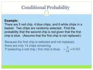
Conditional Probability • Probability of an event given the occurrence of some other event.
Example You’ve been keeping track of the last 1000 emails you received. You find that 100 of them are spam. You also find that 200 of them were put in your junk folder, of which 90 were spam.
Example You’ve been keeping track of the last 1000 emails you received. You find that 100 of them are spam. You also find that 200 of them were put in your junk folder, of which 90 were spam. What is the probability an email you receive is spam?
Example You’ve been keeping track of the last 1000 emails you received. You find that 100 of them are spam. You also find that 200 of them were put in your junk folder, of which 90 were spam. What is the probability an email you receive is spam?
Example You’ve been keeping track of the last 1000 emails you received. You find that 100 of them are spam. You also find that 200 of them were put in your junk folder, of which 90 were spam. What is the probability an email you receive is spam? What is the probability an email you receive is put in your junk folder?
Example You’ve been keeping track of the last 1000 emails you received. You find that 100 of them are spam. You also find that 200 of them were put in your junk folder, of which 90 were spam. What is the probability an email you receive is spam? What is the probability an email you receive is put in your junk folder?
Example You’ve been keeping track of the last 1000 emails you received. You find that 100 of them are spam. You also find that 200 of them were put in your junk folder, of which 90 were spam. What is the probability an email you receive is spam? What is the probability an email you receive is put in your junk folder? Given that an email is in your junk folder, what is the probability it is spam?
Example You’ve been keeping track of the last 1000 emails you received. You find that 100 of them are spam. You also find that 200 of them were put in your junk folder, of which 90 were spam. What is the probability an email you receive is spam? What is the probability an email you receive is put in your junk folder? Given that an email is in your junk folder, what is the probability it is spam?
Example You’ve been keeping track of the last 1000 emails you received. You find that 100 of them are spam. You also find that 200 of them were put in your junk folder, of which 90 were spam. What is the probability an email you receive is spam? What is the probability an email you receive is put in your junk folder? Given that an email is in your junk folder, what is the probability it is spam? Given that an email is spam, what is the probability it is in your junk folder?
Example You’ve been keeping track of the last 1000 emails you received. You find that 100 of them are spam. You also find that 200 of them were put in your junk folder, of which 90 were spam. What is the probability an email you receive is spam? What is the probability an email you receive is put in your junk folder? Given that an email is in your junk folder, what is the probability it is spam? Given that an email is spam, what is the probability it is in your junk folder?
Application to Machine Learning • In machine learning we have a space H of hypotheses: h1 ,h2 , ...,hn(possibly infinite) • We also have a set D of data • We want to calculate P(h | D) • Bayes rule gives us:
Terminology • Prior probability of h: • P(h): Probability that hypothesis h is true given our prior knowledge • If no prior knowledge, all h H are equally probable • Posterior probability of h: • P(h | D): Probability that hypothesis h is true, given the data D. • Likelihood of D: • P(D | h): Probability that we will see data D, given hypothesis h is true. • Marginal likelihood of D
The Monty Hall Problem You are a contestant on a game show. There are 3 doors, A, B, and C. There is a new car behind one of them and goats behind the other two. Monty Hall, the host, knows what is behind the doors. He asks you to pick a door, any door. You pick door A. Monty tells you he will open a door, different from A, that has a goat behind it. He opens door B: behind it there is a goat. Monty now gives you a choice: Stick with your original choice A or switch to C. Should you switch? http://math.ucsd.edu/~crypto/Monty/monty.html
Bayesian probability formulation Hypothesis space H: h1= Car is behind door A h2= Car is behind door B h3= Car is behind door C Data D: After you picked door A, Monty opened B to show a goat What is P(h1 | D)? What is P(h2 | D)? What is P(h3 | D)?
Bayesian probability formulation Prior probability: P(h1) = 1/3 P(h2) =1/3 P(h3) =1/3 Likelihood: P(D| h1) = 1/2 P(D | h2) = 0 P(D | h3) = 1 Marginal likelihood: P(D) = p(D|h1)p(h1) + p(D|h2)p(h2) + p(D|h3)p(h3) = 1/6 + 0 + 1/3 = 1/2 Hypothesis space H: h1= Car is behind door A h2= Car is behind door B h3= Car is behind door C Data D: After you picked door A, Monty opened B to show a goat What is P(h1 | D)? What is P(h2 | D)? What is P(h3 | D)?
By Bayes rule: So you should switch!
MAP (“maximum a posteriori”) Learning Bayes rule: Goal of learning: Find maximum a posteriori hypothesis hMAP: because P(D) is a constant independent of h.
Note: If every h H is equally probable, then hMAPis called the “maximum likelihood hypothesis”.
A Medical Example Toby takes a test for leukemia. The test has two outcomes: positive and negative. It is known that if the patient has leukemia, the test is positive 98% of the time. If the patient does not have leukemia, the test is positive 3% of the time. It is also known that 0.008 of the population has leukemia. Toby’s test is positive. Which is more likely: Toby has leukemia or Toby does not have leukemia?
Hypothesis space: h1 = T. has leukemia h2 = T. does not have leukemia • Prior: 0.008 of the population has leukemia. Thus P(h1) = 0.008 P(h2) = 0.992 • Likelihood: P(+ | h1) = 0.98, P(− | h1) = 0.02 P(+ | h2) = 0.03, P(− | h2) = 0.97 • Posterior knowledge: Blood test is + for this patient.
In summary P(h1) = 0.008, P(h2) = 0.992 P(+ | h1) = 0.98, P(− | h1) = 0.02 P(+ | h2) = 0.03, P(− | h2) = 0.97 • Thus:
What is P(leukemia|+)? So, These are called the “posterior” probabilities.
Bayesianism vs. Frequentism • Classical probability: Frequentists • Probability of a particular event is defined relative to its frequency in a sample space of events. • E.g., probability of “the coin will come up heads on the next trial” is defined relative to the frequency of heads in a sample space of coin tosses. • Bayesian probability: • Combine measure of “prior” belief you have in a proposition with your subsequent observations of events. • Example: Bayesian can assign probability to statement “There was life on Mars a billion years ago” but frequentist cannot.
Independence and Conditional Independence • Two random variables, X and Y, are independent if • Two random variables, X and Y, are independent given C if
Naive Bayes Classifier Let f (x) be a target function for classification: f (x) {+1, −1}. Letx= (x1, x2, ..., xn) We want to find the most probable class value, hMAP, given the data x:
By Bayes Theorem: P(class) can be estimated from the training data. How? However, in general, not practical to use training data to estimate P(x1, x2, ..., xn | class). Why not?
Naive Bayes classifier: Assume Is this a good assumption? Given this assumption, here’s how to classify an instance x = (x1, x2, ...,xn): Naive Bayes classifier:
Naive Bayes classifier: Assume Is this a good assumption? Given this assumption, here’s how to classify an instance x = (x1, x2, ...,xn): Naive Bayes classifier:
Naive Bayes classifier: Assume Is this a good assumption? Given this assumption, here’s how to classify an instance x = (x1, x2, ...,xn): Naive Bayes classifier: To train: Estimate the values of these various probabilities over the training set.
Training data: Day Outlook Temp Humidity Wind PlayTennis D1 Sunny Hot High Weak No D2 Sunny Hot High Strong No D3 Overcast Hot High Weak Yes D4 Rain Mild High Weak Yes D5 Rain Cool Normal Weak Yes D6 Rain Cool Normal Strong No D7 Overcast Cool Normal Strong Yes D8 Sunny Mild High Weak No D9 Sunny Cool Normal Weak Yes D10 Rain Mild Normal Weak Yes D11 Sunny Mild Normal Strong Yes D12 Overcast Mild High Strong Yes D13 Overcast Hot Normal Weak Yes D14 Rain Mild High Strong No Test data: D15 Sunny Cool High Strong ?
Use training data to compute a probabilistic model: Day Outlook Temp Humidity Wind PlayTennis D15 Sunny Cool High Strong ?
Use training data to compute a probabilistic model: Day Outlook Temp Humidity Wind PlayTennis D15 Sunny Cool High Strong ?
Estimating probabilities / Smoothing • Recap: In previous example, we had a training set and a new example, (Outlook=sunny, Temperature=cool, Humidity=high, Wind=strong) • We asked: What classification is given by a naive Bayes classifier? • Let nc be the number of training instances with class c. E.g., nyes= 9 • Let be the number of training instances with attribute value xi=ak and class c. E.g., Then
Problem with this method: If nc is very small, gives a poor estimate. • E.g., P(Outlook = Overcast | no) = 0.
Now suppose we want to classify a new instance: (Outlook=overcast, Temperature=cool, Humidity=high, Wind=strong) Then: This incorrectly gives us zero probability due to small sample.
Day Outlook Temp Humidity Wind PlayTennis D1 Sunny Hot High Weak No D2 Sunny Hot High Strong No D3 Overcast Hot High Weak Yes D4 Rain Mild High Weak Yes D5 Rain Cool Normal Weak Yes D6 Rain Cool Normal Strong No D7 Overcast Cool Normal Strong Yes D8 Sunny Mild High Weak No D9 Sunny Cool Normal Weak Yes D10 Rain Mild Normal Weak Yes D11 Sunny Mild Normal Strong Yes D12 Overcast Mild High Strong Yes D13 Overcast Hot Normal Weak Yes D14 Rain Mild High Strong No Training data: How should we modify probabilities?
One solution: Laplace smoothing (also called “add-one” smoothing) For each class c and attribute xi with value ak, add one “virtual” instance. That is, for each class c, recalculate: where K is the number of possible values of attribute a.
Day Outlook Temp Humidity Wind PlayTennis D1 Sunny Hot High Weak No D2 Sunny Hot High Strong No D3 Overcast Hot High Weak Yes D4 Rain Mild High Weak Yes D5 Rain Cool Normal Weak Yes D6 Rain Cool Normal Strong No D7 Overcast Cool Normal Strong Yes D8 Sunny Mild High Weak No D9 Sunny Cool Normal Weak Yes D10 Rain Mild Normal Weak Yes D11 Sunny Mild Normal Strong Yes D12 Overcast Mild High Strong Yes D13 Overcast Hot Normal Weak Yes D14 Rain Mild High Strong No Training data: Laplace smoothing: Add the following virtual instances for Outlook: Outlook=Sunny: YesOutlook=Overcast: YesOutlook=Rain: Yes Outlook=Sunny: NoOutlook=Overcast: NoOutlook=Rain: No
Naive Bayes on continuous-valued attributes • How to deal with continuous-valued attributes? Two possible solutions: • Discretize • Assume particular probability distribution of classes over values (estimate parameters from training data)
Discretization: Equal-Width Binning For each attribute xi , create k equal-width bins in interval from min(xi ) to max(xi). The discrete “attribute values” are now the bins. Questions: What should k be? What if some bins have very few instances? Problem with balance between discretization bias and variance. The more bins, the lower the bias, but the higher the variance, due to small sample size.
Discretization: Equal-Frequency Binning For each attribute xi , create k bins so that each bin contains an equal number of values. Also has problems: What should k be? Hides outliers. Can group together instances that are far apart.
Gaussian Naïve Bayes Assume that within each class, values of each numeric feature are normally distributed: where μi,cis the mean of feature igiven the class c,and σi,cis the standard deviation of feature igiven the class c We estimate μi,c and σi,cfrom training data.