Download
1 / 18
180 likes | 315 Vues
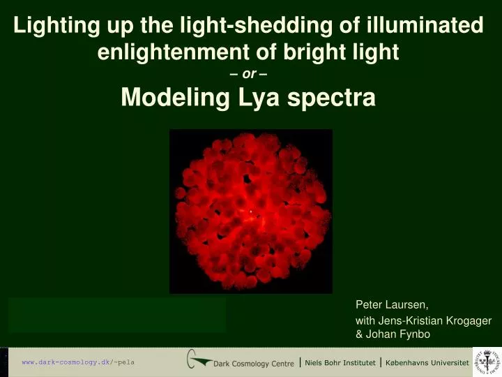
Lighting up the light-shedding of illuminated enlightenment of bright light – or – Modeling Lya spectra. Peter Laursen, with Jens-Kristian Krogager & Johan Fynbo. | Niels Bohr Institutet | Københavns Universitet. www.dark-cosmology.dk /~pela. QSO2222-0946.

E N D
Lighting up the light-shedding of illuminated enlightenment of bright light – or – Modeling Lya spectra Peter Laursen, with Jens-Kristian Krogager & Johan Fynbo | Niels Bohr Institutet | Københavns Universitet www.dark-cosmology.dk/~pela
QSO2222-0946 HST/UVIS with the F606W filter
QSO2222-0946 VLT/X-Shooter (UVB arm)
QSO2222-0946 VLT/X-Shooter (UVB arm)
Modeling Lya lines …has been done before ⇒ Verhamme et al. (2008) with MCLYA
The model MoCaLaTA
Input parameters Geometry: • Radius • Number of clouds • Cloud size distribution MoCaLaTA rgal Ncl rcl,min; rcl,max; β State of the clouds and the intercloud medium: • Neutral hydrogen density • Temperature • Dust density ⇐ metallicity nHI,cl; nHI,ICM THI,cl; THI,ICM ZHI,cl; ZHI,ICM Kinematics: • Cloud velocity dispersion • Outflow velocity sV,cl Vout Emission: • Intrinsic line width • Emission scale length • Emission site/cloud correlation • Systemic redshift sline Hem Pcl z
Input parameters rgal Ncl rcl,min; rcl,max; β 10 kpc Kim+ 03 (LMC) ∼105 Dickey & Garwood 89; Williams & McKee 97 10–100 pc; –1.6 nHI,cl; nHI,ICM THI,cl; THI,ICM ZHI,cl; ZHI,ICM sV,cl Vout sline Hem Pcl z
Input parameters rgal Ncl rcl,min; rcl,max; β 0.2–0.5 cm-3 from e.g. Carilli+ 98; Ferrière 01; Gloeckler & Geiss 04 (MW) 10 kpc ∼105 10–100 pc; –1.6 ntot = 10–3–10–2 cm-3 (Dopita & Sutherland 03; Ferrière 01), xHI,ICM ∼ 10–8–10–5 (House 64; Sutherland & Dopita 93), plus residual diffuse HI clouds. nHI,cl; nHI,ICM THI,cl; THI,ICM ZHI,cl; ZHI,ICM 0.3 cm–3; 10–10–10–5 cm–3 e.g. Brinks+ 00; Tüllmann+ 06,08 106 K 104 K; 0.31 Z From Zn, Si, and Fe abs. lines, as well as from [OII]/[OIII] and [NII]/Ha (R23 and N2 methods) sV,cl Vout sline Hem Pcl z
Input parameters rgal Ncl rcl,min; rcl,max; β 10 kpc ∼105 10–100 pc; –1.6 nHI,cl; nHI,ICM THI,cl; THI,ICM ZHI,cl; ZHI,ICM 0.3 cm–3; 10–10–10–5 cm–3 104 K; 106 K 0.31 Z sV,cl Vout 115±18 km s–1 From abs. line widths 100–200 km s–1 sline Hem Pcl z
Input parameters rgal Ncl rcl,min; rcl,max; β 10 kpc ∼105 10–100 pc; –1.6 nHI,cl; nHI,ICM THI,cl; THI,ICM ZHI,cl; ZHI,ICM 0.3 cm–3; 10–10–10–5 cm–3 104 K; 106 K 0.31 Z sV,cl Vout 115±18 km s–1 100–200 km s–1 sline Hem Pcl z 130 km s–1 From [OII], [OIII], Ha, and Hb 2.1 kpc From HST imaging (reff = 1.09 kpc) n/a 0.2–0.5 2.35 From [OII], [OIII], Ha, and Hb
Input parameters rgal Ncl rcl,min; rcl,max; β Set by observations 10 kpc ∼105 Standard values 10–100 pc; –1.6 Fitted for nHI,cl; nHI,ICM THI,cl; THI,ICM ZHI,cl; ZHI,ICM 0.3 cm–3; 10–10–10–5 cm–3 104 K; 106 K 0.31 Z sV,cl Vout 115±18 km s–1 100–200 km s–1 sline Hem Pcl z 130 km s–1 2.1 kpc n/a 2.35
Finding the best fit 1. Run trial models to get a rough fit ⇒ Ncl∼ 105; Vout∼ 150 km s-1 2. Run grid with Ncl∈ [104.5,105.5] and Vout∈ [100,200] km s-1 ⇒
Finding the best fit 1. Run trial models to get a rough fit ⇒ Ncl∼ 105; Vout∼ 150 km s-1 2. Run grid with Ncl∈ [104.5,105.5] and Vout∈ [100,200] km s-1 3. Fit skewed Gaußians 4. Measure a) Red peak FWHM b) Peak separation c) Peak height ratio d) Peak flux ratio
Finding the best fit 1. Run trial models to get a rough fit ⇒ Ncl∼ 105; Vout∼ 150 km s-1 2. Run grid with Ncl∈ [104.5,105.5] and Vout∈ [100,200] km s-1 3. Fit skewed Gaußians 4. Measure a) Red peak FWHM b) Peak separation c) Peak height ratio d) Peak flux ratio 5. Calculate number of std. dev.sbetween synthetic and observed spectra 6. Identify best fitting model and those for which all four fitting parameters fall within 1σ
Results Best-fitting models give: Vout= 160 km s-1 log(NHI/cm-2) = 20.23 Ncl= 2±1
Results Best-fitting models give: Vout= 160 km s-1 log(NHI/cm-2) = 20.23 Ncl= 2±1
Conclusion • Fitting Lya lines requires information about several parameters. A simple spectrum isn’t really enough.