Download

1 / 47
480 likes | 741 Vues
Motion Planning. Howie CHoset. What is Motion Planning?. Determining where to go. Overview. The Basics Motion Planning Statement The World and Robot Configuration Space Metrics. Algorithms. Start-Goal Methods Map-Based Approaches Cellular Decompositions. The World consists of.

E N D
Motion Planning Howie CHoset
What is Motion Planning? • Determining where to go
Overview • The Basics • Motion Planning Statement • The World and Robot • Configuration Space • Metrics
Algorithms • Start-Goal Methods • Map-Based Approaches • Cellular Decompositions
The World consists of... • Obstacles • Already occupied spaces of the world • In other words, robots can’t go there • Free Space • Unoccupied space within the world • Robots “might” be able to go here • To determine where a robot can go, we need to discuss what a Configuration Space is
Motion Planning Statement If W denotes the robot’s workspace, And Cidenotes the i’th obstacle, Then the robot’s free space, FS, is defined as: FS = W - ( U Ci ) And a path c C0is c : [0,1] g FS where c(0) is qstart and c(1) is qgoal
Free Space Obstacles Robot x,y Example of a World (and Robot)
Basics: Metrics • There are many different ways to measure a path: • Time • Distance traveled • Expense • Distance from obstacles • Etc…
Attractive/Repulsive Potential Field • Uatt is the “attractive” potential --- move to the goal • Urep is the “repulsive” potential --- avoid obstacles
Artificial Potential Field Methods:Attractive Potential Quadratic Potential
The Wavefront Planner • A common algorithm used to determine the shortest paths between two points • In essence, a breadth first search of a graph • For simplification, we’ll present the world as a two-dimensional grid • Setup: • Label free space with 0 • Label start as START • Label the destination as 2
Representations • World Representation • You could always use a large region and distances • However, a grid can be used for simplicity
Representations: A Grid • Distance is reduced to discrete steps • For simplicity, we’ll assume distance is uniform • Direction is now limited from one adjacent cell to another • Time to revisit Connectivity (Remember Vision?)
Representations: Connectivity • 8-Point Connectivity • 4-Point Connectivity • (approximation of the L1 metric)
The Wavefront in Action (Part 1) • Starting with the goal, set all adjacent cells with “0” to the current cell + 1 • 4-Point Connectivity or 8-Point Connectivity? • Your Choice. We’ll use 8-Point Connectivity in our example
The Wavefront in Action (Part 2) • Now repeat with the modified cells • This will be repeated until no 0’s are adjacent to cells with values >= 2 • 0’s will only remain when regions are unreachable
The Wavefront in Action (Part 3) • Repeat again...
The Wavefront in Action (Part 4) • And again...
The Wavefront in Action (Part 5) • And again until...
The Wavefront in Action (Done) • You’re done • Remember, 0’s should only remain if unreachable regions exist
The Wavefront, Now What? • To find the shortest path, according to your metric, simply always move toward a cell with a lower number • The numbers generated by the Wavefront planner are roughly proportional to their distance from the goal Two possible shortest paths shown
Wavefront (Overview) • Divide the space into a grid. • Number the squares starting at the start in either 4 or 8 point connectivity starting at the goal, increasing till you reach the start. • Your path is defined by any uninterrupted sequence of decreasing numbers that lead to the goal.
This is really a Continuous Solution Not pixels Waves bend L1 distance
Free Space Obstacles Robot x,y Example of a World (and Robot)
Free Space Obstacles Robot (treat as point object) x,y Configuration Space: Accommodate Robot Size
What if the robot is not a point? The Scout should probably not be modeled as a point... b a Nor should robots with extended linkages that may contact obstacles...
Configuration Space “Quiz” Where do we put ? 360 qA A 270 b B 180 b 90 a qB a 0 45 135 90 180 An obstacle in the robot’s workspace Torus (wraps horizontally and vertically)
Configuration Space Obstacle How do we get from A to B ? Reference configuration 360 qA A 270 b B 180 b 90 a qB a 0 45 135 90 180 An obstacle in the robot’s workspace The C-space representation of this obstacle…
Two Link Path Thanks to Ken Goldberg
With Rotation: how much distance to rotate Pick a reference point…
The Configuration Space • What it is • A set of “reachable” areas constructed from knowledge of both the robot and the world • How to create it • First abstract the robot as a point object. Then, enlarge the obstacles to account for the robot’s footprint and degrees of freedom • In our example, the robot was circular, so we simply enlarged our obstacles by the robot’s radius (note the curved vertices)
x,y Configuration Space: the robot has... • A Footprint • The amount of space a robot occupies • Degrees of Freedom • The number of variables necessary to fully describe a robot’s configuration in space • You’ll cover this more in depth later • fun with non-holonomic constraints, etc
Translate-only, non-circularly symmetric Pick a reference point…
The Configuration Space • What it is • A set of “reachable” areas constructed from knowledge of both the robot and the world • How to create it • First abstract the robot as a point object. Then, enlarge the obstacles to account for the robot’s footprint and degrees of freedom • In our example, the robot was circular, so we simply enlarged our obstacles by the robot’s radius (note the curved vertices)