Download
1 / 43
450 likes | 645 Vues
Classic AI Search Problems. Sliding tile puzzles 8 Puzzle (3 by 3 variation) Small number of 8!/2, about 1.8 *10 5 states 15 Puzzle (4 by 4 variation) Large number of 16!/2 , about 1.0 *10 13 states 24 Puzzle (5 by 5 variation)

E N D
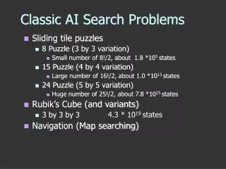
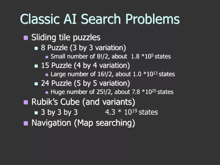
Classic AI Search Problems • Sliding tile puzzles • 8 Puzzle (3 by 3 variation) • Small number of 8!/2, about 1.8 *105 states • 15 Puzzle (4 by 4 variation) • Large number of 16!/2, about 1.0 *1013 states • 24 Puzzle (5 by 5 variation) • Huge number of 25!/2, about 7.8 *1025 states • Rubik’s Cube (and variants) • 3 by 3 by 3 4.3 * 1019 states • Navigation (Map searching)
2 1 3 4 7 6 5 8 Classic AI Search Problems • Invented by Sam Loyd in 1878 • 16!/2, about1013 states • Average number of 53 moves to solve • Known diameter (maximum length of optimal path) of 87 • Branching factor of 2.13
3*3*3 Rubik’s Cube • Invented by Rubik in 1974 • 4.3 * 1019 states • Average number of 18 moves to solve • Conjectured diameter of 20 • Branching factor of 13.35
Navigation Arad to Bucharest start end
Arad Zerind Sibiu Timisoara Oradea Fagaras Arad Rimnicu Vilcea Sibiu Bucharest Representing Search
General (Generic) SearchAlgorithm function general-search(problem, QUEUEING-FUNCTION) nodes = MAKE-QUEUE(MAKE-NODE(problem.INITIAL-STATE)) loop do if EMPTY(nodes) then return "failure" node = REMOVE-FRONT(nodes) if problem.GOAL-TEST(node.STATE) succeeds then return node nodes = QUEUEING-FUNCTION(nodes, EXPAND(node, problem.OPERATORS)) end A nice fact about this search algorithm is that we can use a single algorithm to do many kinds of search. The only difference is in how the nodes are placed in the queue.
Completeness solution will be found, if it exists Time complexity number of nodes expanded Space complexity number of nodes in memory Optimality least cost solution will be found Search Terminology
Breadth first Uniform-cost Depth-first Depth-limited Iterative deepening Bidirectional Uninformed (blind) Search
QUEUING-FN:- successors added to end of queue (FIFO) Arad Zerind Sibiu Timisoara Oradea Fagaras Arad Rimnicu Vilcea Arad Arad Oradea Lugoj Breadth first
Complete ? Yes if branching factor (b) finite Time ? 1 + b + b2 + b3 +…+ bd = O(bd), so exponential Space ? O(bd), all nodes are in memory Optimal ? Yes (if cost = 1 per step), not in general Properties of Breadth first
Assuming b = 10, 1 node per ms and 100 bytes per node Properties of Breadth first cont.
QUEUING-FN:- insert in order of increasing path cost Arad 75 118 140 Zerind Sibiu Timisoara 140 151 99 80 Oradea Fagaras Arad Rimnicu Vilcea 118 75 71 111 Arad Arad Lugoj Oradea Uniform-cost
Complete ? Yes if step cost >= epsilon Time ? Number of nodes with cost <= cost of optimal solution Space ? Number of nodes with cost <= cost of optimal solution Optimal ?- Yes Properties of Uniform-cost
QUEUING-FN:- insert successors at front of queue (LIFO) Arad Zerind Zerind Sibiu Sibiu Timisoara Timisoara Arad Oradea Depth-first
Complete ? No:- fails in infinite- depth spaces, spaces with loops complete in finite spaces Time ? O(bm), bad if m is larger than d Space ? O(bm), linear in space Optimal ?:- No Properties of Depth-first
Choose a limit to depth first strategy e.g 19 for the cities Works well if we know what the depth of the solution is Otherwise use Iterative deepening search (IDS) Depth-limited
Complete ? Yes if limit, l >= depth of solution, d Time ? O(bl) Space ? O(bl) Optimal ? No Properties of depth limited
Iterative deepening search (IDS) function ITERATIVE-DEEPENING-SEARCH(): for depth = 0 to infinity do if DEPTH-LIMITED-SEARCH(depth) succeeds then return its result end return failure
Complete ? Yes Time ? (d + 1)b0 + db1 + (d - 1)b2 + .. + bd = O(bd) Space ? O(bd) Optimal ? Yes if step cost = 1 Properties of IDS
Various uninformed search strategies Iterative deepening is linear in space not much more time than others Use Bi-directional Iterative deepening were possible Summary
Island Search Suppose that you happen to know that the optimal solution goes thru Rimnicy Vilcea…
Island Search Suppose that you happen to know that the optimal solution goes thru Rimnicy Vilcea… Rimnicy Vilcea
A* Search • Uses evaluation function f = g+ h • g is a cost function • Total cost incurred so far from initial state • Used by uniform cost search • h is an admissible heuristic • Guess of the remaining cost to goal state • Used by greedy search • Never overestimating makes h admissible
A* Our Heuristic
QUEUING-FN:- insert in order of f(n) = g(n) + h(n) Zerind Sibiu Timisoara A* Arad g(Zerind) = 75 g(Timisoara) = 118 g(Sibiu) = 140 g(Timisoara) = 329 h(Zerind) = 374 h(Sibiu) = 253 f(Sibui) = … f(Zerind) = 75 + 374
Properties of A* • Optimal and complete • Admissibility guarantees optimality of A* • Becomes uniform cost search if h= 0 • Reduces time bound from O(b d ) to O(b d - e) • b is asymptotic branching factor of tree • d is average value of depth of search • e is expected value of the heuristic h • Exponential memory usage of O(b d ) • Same as BFS and uniform cost. But an iterative deepening version is possible … IDA*
IDA* • Solves problem of A* memory usage • Reduces usage from O(b d ) to O(bd ) • Many more problems now possible • Easier to implement than A* • Don’t need to store previously visited nodes • AI Search problem transformed • Now problem of developing admissible heuristic • Like The Price is Right, the closer a heuristic comes without going over, the better it is • Heuristics with just slightly higher expected values can result in significant performance gains
A* “trick” • Suppose you have two admissible heuristics… • But h1(n) > h2(n) • You may as well forget h2(n) • Suppose you have two admissible heuristics… • Sometimes h1(n) > h2(n) and sometimes h1(n) < h2(n) • We can now define a better heuristic, h3 • h3(n) = max( h1(n) , h2(n) )
What different does the heuristic make? • Suppose you have two admissible heuristics… • h1(n) is h(n) = 0 (same as uniform cost) • h2(n) is misplaced tiles • h3(n) is Manhattan distance
Game Search (Adversarial Search) • The study of games is called game theory • A branch of economics • We’ll consider special kinds of games • Deterministic • Two-player • Zero-sum • Perfect information
Games • A zero-sum game means that the utility values at the end of the game total to 0 • e.g. +1 for winning, -1 for losing, 0 for tie • Some kinds of games • Chess, checkers, tic-tac-toe, etc.
Problem Formulation • Initial state • Initial board position, player to move • Operators • Returns list of (move, state) pairs, one per legal move • Terminal test • Determines when the game is over • Utility function • Numeric value for states • E.g. Chess +1, -1, 0
Game Trees • Each level labeled with player to move • Max if player wants to maximize utility • Min if player wants to minimize utility • Each level represents a ply • Half a turn
Optimal Decisions • MAX wants to maximize utility, but knows MIN is trying to prevent that • MAX wants a strategy for maximizing utility assuming MIN will do best to minimize MAX’s utility • Consider minimaxvalue of each node • Utility of node assuming players play optimally
Minimax Algorithm • Calculate minimax value of each node recursively • Depth-first exploration of tree • Game tree (aka minimax tree) Max node Min node
Min 2 7 5 5 6 7 Example Max 5 4 2 5 10 4 6 Utility
Minimax Algorithm • Time Complexity? • O(bm) • Space Complexity? • O(bm) or O(m) • Is this practical? • Chess, b=35, m=100 (50 moves per player) • 3510010154 nodes to visit
Alpha-Beta Pruning • Improvement on minimax algorithm • Effectively cut exponent in half • Prune or cut out large parts of the tree • Basic idea • Once you know that a subtree is worse than another option, don’t waste time figuring out exactly how much worse
Alpha-Beta Pruning Example 3 2 3 0 3 30 a pruned 32 a pruned 3 5 2 0 5 3 53 b pruned 3 5 1 2 2 0 2 1 2 3 5 0