Download
1 / 26
260 likes | 390 Vues
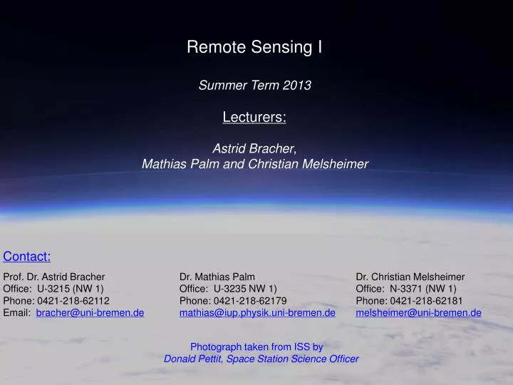
Remote Sensing I Summer Term 2013 Lecturers: Astrid Bracher , Mathias Palm and Christian Melsheimer Contact: Prof. Dr. Astrid Bracher Dr . Mathias Palm Dr. Christian Melsheimer Office: U-3215 (NW 1) Office: U-3235 NW 1) Office: N-3371 (NW 1)

E N D
Remote Sensing I Summer Term 2013 Lecturers: Astrid Bracher, Mathias Palm and Christian Melsheimer Contact: Prof. Dr. Astrid BracherDr. Mathias Palm Dr. Christian Melsheimer Office: U-3215 (NW 1) Office: U-3235 NW 1) Office: N-3371 (NW 1) • Phone: 0421-218-62112 Phone: 0421-218-62179 Phone: 0421-218-62181 Email: bracher@uni-bremen.demathias@iup.physik.uni-bremen.demelsheimer@uni-bremen.de Photograph taken from ISS by Donald Pettit, Space Station Science Officer
Outline Lecture 1Introduction& EM Radiation 04.04.2013 Bracher Lecture 2 EMR II & RadiativeTransfer 11.04.2013 Bracher Lecture 3RetrievalTechniques, Inverse Methods 18.04.2013 Palm Lecture 4SatelliteRemote Sensing (RS) 25.04.2013Bracher Lecture5Spectroscopy02.05.2013 Bracher Lecture 6Infra-redTechniques 16.05.2013 Palm Lecture 7 UV-visibleAtmospheric RS I 23.05.2013Bracher Lecture 8 UV-visibleAtmospheric RS II 30.05.2013 Bracher Lecture 9OceanOptics06.06.2013Bracher Lecture 10Ocean Color Remote Sensing 13.06.2013 Bracher Lecture 11Microwave RS 20.06.2013Palm Lecture12SeaIce Remote Sensing27.06.2013Melsheimer Lecture13 Summary & Lab Tour04.07.2013 Bracher/MW Group Exam: 11 July 2013 10-12
Geostationary orbit • Circular orbit in the equatorial plane, altitude ~36,000km • Orbital period ~1 day , orbit matches Earth’s rotation Advantages • See whole Earth disk at once due to large distance • See same spot on the surface all the time i.e. high temporal coverage • Big advantage for weather monitoring satellites (knowing the atmospheric dynamics is critical to short-term forecasting and numerical weather prediction - NWP) • Disadvantages • Low spatial resolution
Geostationary orbit Meteorological satellites: A combination of OES-E, GOES-W, METEOSAT (Eumetsat), GMS (NASDA), IODC (old Meteosat 5) GOES 1st gen. (GOES-1 - ’75 GOES-7 ‘95); 2nd gen. (GOES-8++ ‘94)
Geostationary orbit METEOSAT - whole earth disk every 15 mins
Orbital Disadvantages ofGEO • typically low spatial resolution due to high altitude: e.g. METEOSAT 2nd Generation (MSG) 1 kmx1 km visible, 3 kmx3 km IR (used to be 3 x 3 & 6 x 6, respectively) • spatial resolution at 60-70° several times lower • not much good beyond 70°- cannot see the poles very well (orbit over equator) Other geosynchronous orbits which are not GEO: same period as Earth, but not equatorial
Lower Earth Orbit (LEO):Polar & near polar orbits Advantages • full polar orbit inclined 90° to equator • typically few degrees off, so poles not covered • orbital period, T, typically 90 – 110 min • near circular orbit between 300 km and 1000 km (low Earth orbit) • typically higher spatial resolution than geostationary • rotation of Earth under satellite gives (potential) total coverage • ground track repeat typically 14-16 days
Lower Earth Orbit (LEO) Ground track of SCIAMACHY (on ENVISAT with 98° inclination and 780 km orbit height) nadir at 1 day
Sun elevation at local noon Sun elevation angle at local noon at the four seasons 21 Dec 21 Mar/22 Sep 21 Jun Bremen, 53°N 14° 37.5° 61° Delhi, 28°N 39° 63° 85° Singapore, 1°N 65.5° 90° 67.5° (over S horizon) (zenith) (over N horizon)
Lower Earth Orbit (LEO):Inclination (tropical) orbits • orbit inclined >0° to <90° to equator • Determined by the region of Earth that is of most interest (e.g. low inclination angle for tropics) • Orbital altitude typically a few hundreds km • Orbital period around a few hours • These satellites are not sun-synchronous view a place on Earth at varying times
Lower Earth Orbit (LEO) Orbital Disadvantages forLEO • need to launch to precise altitude and orbital inclination • orbital decay at LEOs (Low Earth Orbits) < 1000 km • drag from atmosphere causes orbit to become more eccentric • drag increases with increasing solar activity (sun spots) • ~ solar maximum (~11yr cycle) drag height increased by 100km!
Instrument’s Swath Swath describes ground area imaged by instrument during overpass
Lower Earth Orbit (LEO) Ground track of SCIAMACHY (on ENVISAT with 98° inclination and 780 km orbit height) nadir at 1 day
ENVISAT: 1 March 2002 - 12 Apr 2012) • SCIAMACHY • UV/Vis/NIR gratingspectrometers: • 8 channels, 240 - 2380 nm • Moderate spectral resolution: 0.2 – 1.5 nm • Measurement Geometries : • nadir viewing+ limb + solar / lunar occultation • Polar, sun-synchronous orbit, 10:00 • Global coverage in 6 days • During eclipse calibration and limb measurements • Spectroscopy is used to derive trace gas distributions in the troposphere, stratosphere and mesosphere
Overview of satellite observations geometries Overview of satellite observations geometries Measured signal: Directly transmitted solar radiation (Thermal emission from Earth) Measured signal: Reflected and scattered sunlight (Thermal emission from Earth) Measured signal: Scattered solar radiation (Thermal emission from Earth)
Instrument’s Swath Swath describes ground area imaged by instrument during overpass
MODIS: Note across-track “whiskbroom” type scanning mechanism swath width of 2330 km (250-1000m resolution) Hence, 1-2 day repeat cycle Broad Swath • MODIS, POLDER, AVHRR etc. • swaths typically several 1000s of km • lower spatial resolution • Wide area coverage • Large overlap obtains many more view and illumination angles (much better BRDF sampling) • Rapid repeat time
Narrow Swath • Landsat TM/MSS/ETM+, IKONOS, QuickBird etc. • swaths typically few 10s to 100s km • higher spatial resolution • local to regional coverage NOT global • far less overlap (particularly at lower latitudes) • May have to wait weeks/months for revisit Landsat: • 185km swath width, hence 16-day repeat cycle (and spatial res. 25m) • Contiguous swaths overlap (sidelap) by 7.3% at the equator • Much greater overlap at higher latitudes (80% at 84°)
Single or multiple observations How far apart are observations in time? One-off, several or many? Depends (as usual) on application Is it dynamic? If so, over what timescale? Examples Vegetation stress monitoring, weather, rainfall hours to days Terrestrial carbon, ocean surface temperature days to months to years Glacier dynamics, ice sheet mass balance Months to decades What temporal resolution chosen for measurements?
Sensor orbit geostationary orbit – good temporal sampling over same spot: BUT due to large orbit height nearly the entire hemisphere can be viewed (e.g. METEOSAT) Near-polar orbit – less temporal sampling, but can use Earth rotation to view entire surface Sensor swath Wide swath allows more rapid revisit typical are moderate resolution instruments for regional/global applications Narrow swath == longer revisit times typical of higher resolution for regional to local applications What determines the temporal sampling
Coverage (hence spatial and/or temporal sampling) due to combination of orbit and swath Mostly swath - many orbits nearly same MODIS and Landsat have identical orbital characteristics: Inclination 98.2°, h=705 km, T = 99mins BUT swaths of 2400 km and 185 km, repeat of 1-2 days and 16 days, respectively Most EO satellites typically near-polar orbits with repeat tracks every 16 or so days BUT wide swath instrument can view same spot much more frequently than narrow Tradeoffs again, as a function of objectives Summary: spatial and temporal resolution