Download
1 / 48
490 likes | 538 Vues
Learn about Adaptively Sampled Distance Fields (ADFs), a data structure that represents shapes beyond 3D geometry, storing auxiliary data and enabling efficient rendering and operations. Explore the benefits, methods, applications, and advantages of ADFs.

E N D
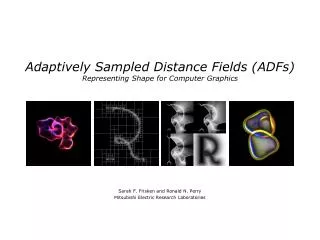
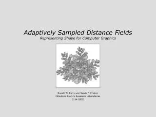
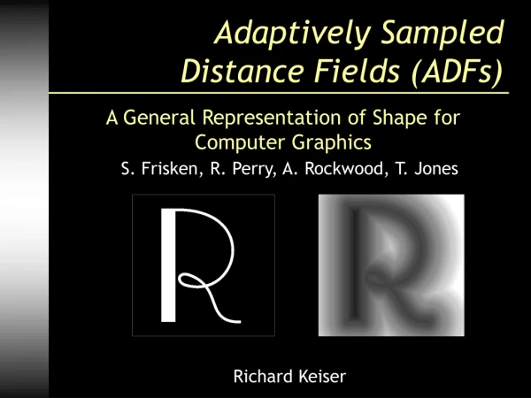
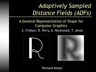
Adaptively Sampled Distance Fields (ADFs) A General Representation of Shape for Computer Graphics S. Frisken, R. Perry, A. Rockwood, T. Jones Richard Keiser
Contents • Introduction • What are ADFs • Motivation • Why is it a hard problem • Idea and Methods • Distance fields • Octree-based ADFs • Algorithms • Applications • Results • Personal statement
Introduction ... or what it‘s all about
What are ADFs ? • A unifying data structure • Represents shapes • More than just the 3D geometry of physical objects • Shape can have arbitrary dimension and be derived from simulated or measured data. • Represents sharp edges, organic surfaces, semi-transparent substances • Can store auxiliary data in cells • Fundamental graphical data structure
Rendering Volume Data • Example : Cocaine molecule volume rendered in a haze of turbulent mist • Color function of mist is based on the distance from the molecule surface • Modulated by a noise function
Shape Representations • Parametric surfaces • Polygons, spline patches, trimmed NURBs • Need associated data structures (B-reps) • Do not represent object interiors or exteriors • Subdivision surfaces • The same disadvantages as parametric surfaces • Implicit surfaces • Defined by an implicit function f(x) = c • Distinguish between interior and exterior • Difficult to define for an arbitrary object
Motivation ... or why it‘s worth listening
Why is it a Hard Problem ? This limitations and problems are addressed by ADFs • Resolution limited by the sampling rate • Large volume size (memory) • Efficiency • Interpolation of the normals of surface points from the sampled data • Expensive and with limited accuracy
Advantages of ADFs • Representing a broad class of forms • Efficient rendering • Efficient and easy use of operations • Locating surface points, performing inside/outside and proximity tests, Boolean operations, blending, closest points, ... • Adaptive sampling -> accuracy • Efficient memory usage
Idea and Methods ... or how it works
Distance Fields • Scalar field that specifies the minimum distance to a shape • At each sample point, store the signed distance to the nearest surface point • Sign indicates inside vs. outside • This sampled distance field is a distance map • Effective representation of shape
Examples • Unit sphere S in R3 • Euclidean signed distance from S :h(x) = 1 - (x2+y2+z2)1/2 • Algebraic signed distance from S :h(x) = 1 - (x2+y2+z2) z P1 h > 0 h < 0 P2 y x r=1
Examples • Implicit form of an object • Euclidean dist. to a parametric surface • distance field computed for a 32 bicubic Bezier patch of the Utah Teapot • Determined by solving the 7th order Bezier equations using the Bezier clipping algorithm
Distance Maps • Vary smoothly across surfaces • Are defined throughout space • Can be reconstructed as the zero-value iso-surface of the distance map • Can locally estimate the surface normal by the gradient of the distance map
Gradient Vectors The distance field varies smoothly across the edge The gradient of the distance field accurately estimates the edge normal
Regularly vs. Adaptiv • Regularly sampled distance fields • Large volume size because fine detail requires dense sampling • Adaptively sampled distance fields • Use adaptive, detail-directed sampling • High sampling rates in regions containing fine detail • Store the sampled data in a hierarchy for fast localization
Octree-based ADFs • One possibility for a hierarchy in 3D • Demonstrate the concepts in 2D (with quadtrees) • Quadtree cell • Contains the sampled distance values of the cell‘s 4 corners • Pointers to parent and child cells
Example of a Quadtree c11 c10 c0 c13 c12 c31 c30 SW NE c2 c32 c33 SE NW c0 c2 c33 c32 c31 c30 c13 c12 c11 c10
3-color Quadtree vs. ADFs • 3-color quadtree • 3 types of cells: interior, exterior, boundary • Subdivide all boundary cells to a predetermined highest resolution level • ADFs quadtree • Subdivision of boundary cells depends on the distance field • Subdivide only when the distance field within a cell is not well approximated by bilinear interpolation of its corner values
3-color Quadtree vs. ADFs 3-color quadtree ADFs quadtree 23‘573 cells 1‘713 cells
2D Spatial Data Structure • Wavelet
Generating ADFs • Function to produce the distance function, h(x) • Continuity, differentiablility and bounded growth advantageous, but not necessary • Many ways to generate an ADFs • E.g. bottom-up approach • E.g. top-down approach
Bottom-up Algorithm • Start with a regularly sampled distance field of finite resolution • Construct a fully populated octree (3D) • Repeat (start with the smallest cells) • Coalesce a group of 8 neighbour cells iff • None of the cells has any child cells • sampled distances of all 8 cells reconstructed from the sample values of their parent • Next level Until no cells are coalesced
Top-down Algorithm • Compute the distance values for the root node • Subdivide ADFs cells recursively according to a subdivision rule • e.g. for representing the iso-surface stop if • the cell is guaranteed to not contain the surface • a specified maximum level is reached • the cell contains the surface but can be interpolated to a specified error tolerance
Top-down Generation Initialize root cell Recursively subdivide
Reconstructing ADFs • Distance values within a cell are reconstructed from the stored 8 corner distance values using trilinear interpolation • Surface normal is equal to the normalized gradient of the distance field
Application: Ray Casting • Determine surface points • Intersection between a ray and the zero-value iso-surface of the ADFs • Linear approximation
Application: Ray Casting • Determine the distance values where the ray enters and exits the cell • Compute the crossing if the two values have different signs
Application: Level of Detail • Truncate the ADF-octree at fixed levels: • During rendering, generation, or to an existing high resolution • Can be used for progressive representation • Truncate cells with little errors • Error stored during top-down generation • Consistent degradation for both smooth and highly curved portions of the surface • Can be used for local refinement
Application: Level of Detail Four LOD models with varying amounts of error rendered from an ADFs octree
Application: Collisions • Collision avoidance in robotics • Using distance fields • Penetration forces in haptics • Accelerate collision detection • Using octrees • LOD
Results ...or what we have reached
Conclusions • Adaptively sampling of the distance field • Efficient use of memory • High frequency components are reconstructed accurately • Storing sampled values in a spatial hierarchy • Efficient reconstruction/localization
Triangles vs. ADFs Error Tolerance Triangle Count ADF Cell Count ADF Sample Count 6.25E-5 3.13E-5 1.56E-5 32‘768 131‘072 2‘097‘152 16‘201 44‘681 131‘913 24‘809 67‘405 165‘847 Comparison of triangle count for a sphere (r=0.4) to ADF size
Conclusions • Distance fields embody considerable information about a shape • Inside vs. outside, gradient and proximity information • Operations on a shape often achieved by operations on its distance field -> more efficient
Conclusions • Separate generation of shapes • Preprocessing : complex and time-consuming methods • Runtime : fast graphical operations • Complex shapes can be processed as quickly as much simpler shapes • Fractals, mathematically sophisticated or carved shapes
Conclusions • ADFs integrate numerous concepts in computer graphics • Representation of geometry and volume data • Broad range of processing operations such as rendering, carving, LOD management, surface offsetting, and proximity testing
Conclusion • 2D editing with boolean difference
Personal Statement ...or the paper under my loup
Last Thoughts • ADFs combine known concepts • Advantages • Distance fields -> flexibility • Octrees -> fast location • Adaptation -> accuracy, memory efficiency
Last Thoughts • Disadvantages • Finding a distance function can be difficult • Bottom-up algorithm requires excessive amount of memory • Top-down algorithm performs expensive octree neighbour searches • Main application area • Complex shapes, shapes with fine details
Last Thoughts • Convincing pictures and comparisons • Idea of ADFs and implementation rather easy • Many advantages • Useful for many fundamental graphical operations • propose ADFs as a fundamental graphical data structure
The End ...or are there any questions ?