Download
1 / 51
560 likes | 1.02k Vues
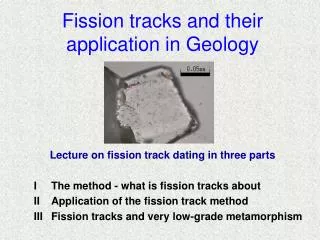
Part - II. Application of the fission track method in Geology. 3 key questions. What geologic questions can be answered? What sampling strategy is required? How can we interpret our fission track data?. Part 2 - The application.

E N D
Part - II Application of the fission track method in Geology
3 key questions What geologic questions can be answered? What sampling strategy is required? How can we interpret our fission track data? Part 2 - The application
What are the processes that we can "date" with fission track data? Very fast processes with rock cooling:volcanic eruptions, intrusions with fast cooling, hydrothermal event, shear heating along fault plane Fast processes with rock cooling:fast exhumation or erosion in an active orogen, fast movements along faults (e.g. tectonic unroofing) Moderately fast processes with rock cooling:moderate exhumation or erosion, moderately cooling in and around intrusive body, Slow processes with rock cooling:slow erosion or exhumation in a decaying orogen Part 2 - The application
Real "dating" with the FT method Only with fast to very fast cooling, the fission track method is able to "date an event" Potential events: • volcanic eruption • fast cooling intrusion • impact event • hydrothermal event • shear heating along thrust plane Part 2 - The application
Process rate estimation with the FT method With moderate and slow cooling, the fission track method only estimates cooling rates. It does NOT necessarily mean an "event". Possible processes: • erosive denudation • tectonic denudation • topography formation • thermal relaxation Part 2 - The application
Fission track dating of a single event - I Australian tektite Glass drops ejected from German impact crater Part 2 - The application
Fission track dating of a single event - II Bohemian Glass from 1849 with 1% of U can be dated with FT check of the fission decay constant Part 2 - The application
Comparison between dating methods - I Example from German volcano (Kraml et al., in prep.): apatite FT data Part 2 - The application
Comparison between dating methods - II Example from German volcano (Kraml et al., in prep.): Part 2 - The application
Comparison between dating methods - II Part 2 - The application
FT dating and anthropology Titanite 0.306 ± 0.056 Ma Thermoluminescence 0.292 ± 0.026 Ma 0.312 ± 0.028 Ma U-series dating 0.300 ± 0.040 Ma Titanite 0.462 ± 0.045 Ma (Guo et al. 1991) Part 2 - The application
How do we know that the FT age represents a single event ? Track length distribution:All tracks are long (mean length > 14.5 mm) and the track length distribution is very narrow. Radial plot:All single grain ages plot in a narrow cluster (except for very young ages or grains with low U content). Statistical tests:The calculated central age passes Poissonian c2 tests. Isochrons:The FT age is in agreement with ages from other dating techniques (e.g. U/Pb, Ar/Ar, (U-Th)/He). Absence of regional variation:The FT age is identical within the same material, also if sampled at other localities. Part 2 - The application
Nanga Parbat - I 100 km Part 2 - The application
Fast exhumation processes: example Nanga Parbat - II 25 km Part 2 - The application
Fast exhumation processes: example Nanga Parbat - III Part 2 - The application
Fast exhumation processes: example Nanga Parbat - IV Part 2 - The application
Fast exhumation processes: example Nanga Parbat - V From: Brozovic et al. (1997) apatite FT ages: A: 0-1 Ma B: 1-6 Ma C: 6-15 Ma Part 2 - The application
Fast exhumation processes: example Taiwan - I from Dadson et al. (2003):Exhumation rates (mm yr-1) based on apatite FT ages:red: reset FT ageorange: partially resetblue: not reset Part 2 - The application
Fast exhumation processes: example Taiwan - II from Dadson et al. (2003):Bedrock incision rates (mm yr-1) as derived from age dating of fluvial terraces much larger than exhumation rates ! Part 2 - The application
Chicken or egg? The main question in research today: Who was first, erosion or tectonics ? How can we know ? • regional plate tectonic context • very fast cooling points to tectonics • climatic evidence • accompagnying processes • topography analysis Part 2 - The application
Uplift - Exhumation - Denudation (England & Molnar 1990) Part 2 - The application
The effect of topography Part 2 - The application
Convex and concave T-t paths Assumption: topography evolves in a vertical direction only, no lateral valley shift Part 2 - The application
The effect of fluid flow (from Kohl & Rybach, www.gtr. geophys.ethz.ch/ neatpiora.html) Part 2 - The application
Fault planes and ages Part 2 - The application
Fault movements in the Central Alps Part 2 - The application
Exhumation in a cratonic continent - I (Gleadow et al. 2002) Part 2 - The application
Exhumation in a cratonic continent - II (Gleadow et al. 2002) 2750 apatite FT ages Part 2 - The application
Exhumation in a cratonic continent - III (Gleadow et al. 2002) Part 2 - The application
Exhumation in a cratonic continent - IV (Gleadow et al. 2002) Part 2 - The application
The principles of fission track data modelling Part 2 - The application
The modelling of FT data: age and track length Part 2 - The application
Genetic algorithm and shrinking of T-t-boxes Part 2 - The application
Why are detrital zircons better than apatites? Part 2 - The application
The lag time concept Part 2 - The application
orogenic cycle Part 2 - The application
Uplift - erosion - topography Davis (1899): uplift is short-term process Penck (1953): uplift is „waxing-waning“ Hack (1975): uplift and topography form steady-state Part 2 - The application
Detrital age spectra: static and younging age components steady age component younging age component Part 2 - The application
raw data with error envelope Probability density plots of FT ages statistical fit to density plot fitted age populations (from Garver et al. 1999) Part 2 - The application
Decrease and increase of lag time (from Bernet et al. 2001) Part 2 - The application
Example: European Alps pro-wedge retro-wedge Part 2 - The application
Example for a decrease of lag time (from Bernet et al. 2004) Part 2 - The application
Example for a steady lag time (from Bernet et al. 2004) Part 2 - The application
FT ages along vertical bore hole Part 2 - The application
FT age evolution along vertical bore hole Part 2 - The application
FT age evolution along vertical bore hole Part 2 - The application
FT age evolution along vertical bore hole Part 2 - The application
example I: bore hole @ Hünenberg (from Cederbom et al., in press) Part 2 - The application
example II: Rigi Mountain and bore hole @ Weggis (from Cederbom et al., in press) Part 2 - The application
Exhumed PAZ at Denali, Alaska (Fitzgerald et al. 1995) Part 2 - The application