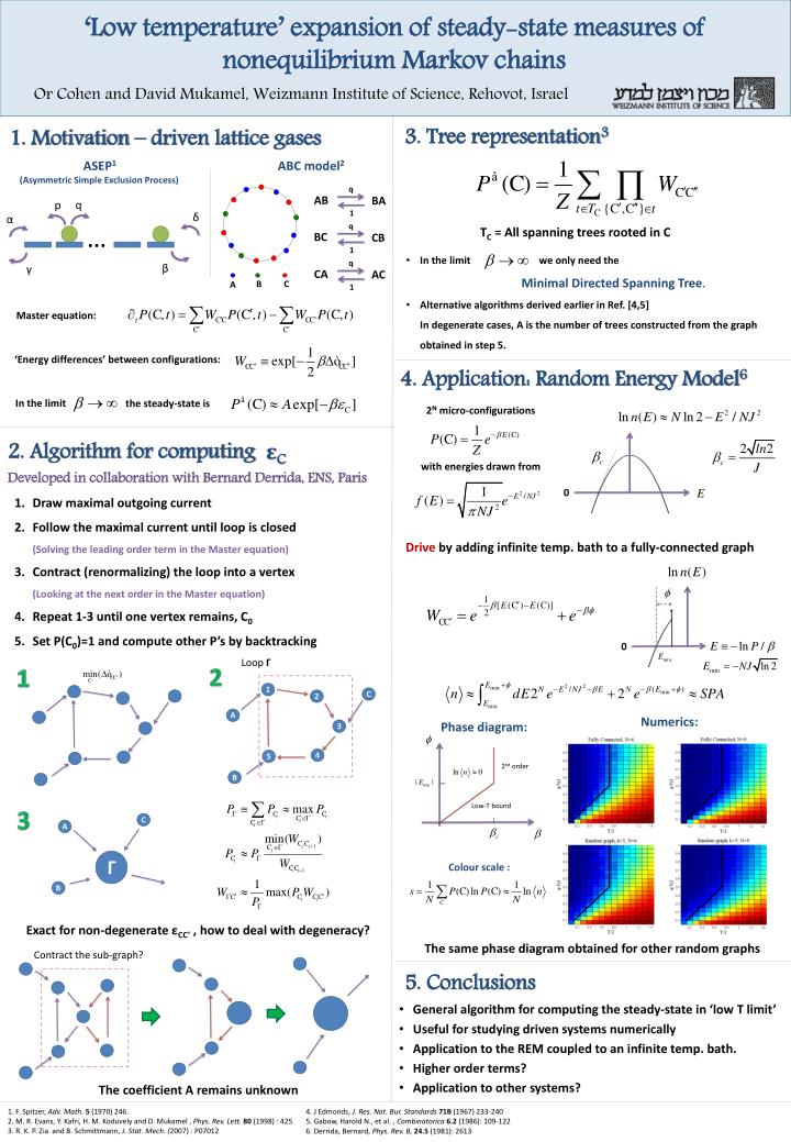
‘Low temperature’ expansion of steady-state measures of nonequilibrium Markov chains

1. B C A ‘Low temperature’ expansion of steady-state measures of nonequilibrium Markov chains Or Cohen and David Mukamel, Weizmann Institute of Science, Rehovot, Israel 3. Tree representation3 1. Motivation – driven lattice gases q p ASEP1 (Asymmetric Simple Exclusion Process) ABC model2 δ α … q AB BA 1 β γ TC = All spanning trees rooted in C q BC CB 1 • In the limit we only need the Minimal Directed Spanning Tree. • Alternative algorithms derived earlier in Ref. [4,5]In degenerate cases, A is the number of trees constructed from the graph obtained in step 5. q CA AC 1 Master equation: ‘Energy differences’ between configurations: 4. Application: Random Energy Model6 In the limit the steady-state is 2N micro-configurations 2. Algorithm for computing εC with energies drawn from Developed in collaboration with Bernard Derrida, ENS, Paris 0 • Draw maximal outgoing current • Follow the maximal current until loop is closed(Solving the leading order term in the Master equation) • Contract (renormalizing) the loop into a vertex(Looking at the next order in the Master equation) • Repeat 1-3 until one vertex remains, C0 • Set P(C0)=1 and compute other P’s by backtracking Drive by adding infinite temp. bath to a fully-connected graph Loop Γ 2 1 1 C 2 0 A Numerics: Phase diagram: 3 4 5 B 3 C A 2nd order Γ Colour scale : Low-T bound B Exact for non-degenerate εCC’ , how to deal with degeneracy? The same phase diagram obtained for other random graphs Contract the sub-graph? 5. Conclusions • General algorithm for computing the steady-state in ‘low T limit’ • Useful for studying driven systems numerically • Application to the REM coupled to an infinite temp. bath. • Higher order terms? • Application to other systems? The coefficient A remains unknown 1. F. Spitzer, Adv. Math.5 (1970) 246. 2. M. R. Evans, Y. Kafri, H. M. Koduvely and D. Mukamel, Phys. Rev. Lett. 80 (1998) : 425 3. R. K. P. Zia and B. Schmittmann, J. Stat. Mech. (2007) : P07012 4. J Edmonds, J. Res. Nat. Bur. Standards71B (1967) 233-240 5. Gabow, Harold N., et al. ,Combinatorica6.2 (1986): 109-122 6. Derrida, Bernard, Phys. Rev. B,24.5 (1981): 2613