Download
1 / 23
230 likes | 398 Vues
Robin Hogan Julien Delano ë , Nicola Pounder, Nicky Chalmers, Thorwald Stein, Anthony Illingworth University of Reading. Synergistic cloud retrievals from radar, lidar and radiometers. Spaceborne radar, lidar and radiometers. The A-Train CloudSat 94-GHz radar (launch 2006)

E N D
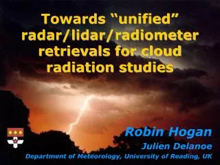
Robin Hogan JulienDelanoë, Nicola Pounder, Nicky Chalmers, Thorwald Stein, Anthony Illingworth University of Reading Synergistic cloud retrievals from radar, lidar and radiometers
Spaceborne radar, lidar and radiometers The A-Train • CloudSat 94-GHz radar (launch 2006) • Calipso 532/1064-nm depol. lidar • MODIS multi-wavelength radiometer • CERES broad-band radiometer • 700-km orbit • NASA EarthCare • EarthCARE (launch 2013) • 94-GHz Doppler radar • 355-nm HSRL/depol. lidar • Multispectral imager • Broad-band radiometer • 400-km orbit (more sensitive) • ESA+JAXA
Towards assimilation of cloud radar and lidar • Before we assimilate radar and lidar into NWP models it is helpful to first develop variational cloud retrievals • Need to develop forward models and their adjoints: used by both • Refine microphysical and a-priori assumptions • Get an understanding of information content from observations • Progress in our development of synergistic radar-lidar-radiometer retrievals of clouds: • Variational retrieval of ice clouds applied to ground-based radar-lidar and the SEVIRI radiometer (Delanoe and Hogan 2008) • Applied to >2 years of A-Train data (Delanoe and Hogan 2010) • Fast forward models for radar and lidar subject to multiple scattering (Hogan 2008, 2009; Hogan and Battaglia 2009) • With ESA & NERC funding, currently developing a “unified” algorithm for retrieving cloud, aerosol and precipitation properties from the EarthCARE radar, lidar and radiometers; will apply to other platforms
Overview • Retrieval framework • Minimization techniques: Gauss-Newton vs. Gradient Descent • Results from CloudSat-Calipso ice-cloud retrieval • Components of unified retrieval: state variables and forward models • Multiple scattering radar and lidar forward model • Multiple field-of-view lidar retrieval • First results from prototype unified retrieval
1. New ray of data: define state vector Use classification to specify variables describing each species at each gate Ice: extinction coefficient , N0’, lidar extinction-to-backscatter ratio Liquid: extinction coefficient and number concentration Rain: rain rate and mean drop diameter Aerosol: extinction coefficient, particle size and lidar ratio 6. Iteration method Derive a new state vector Either Gauss-Newton or quasi-Newton scheme Retrieval framework 2. Convert state vector to radar-lidar resolution Often the state vector will contain a low resolution description of the profile 3. Forward model 3a. Radar model Including surface return and multiple scattering 3c. Radiance model Solar and IR channels 3b. Lidar model Including HSRL channels and multiple scattering Ingredients developed before In progress Not yet developed Not converged 4. Compare to observations Check for convergence 5. Convert Jacobian/adjoint to state-vector resolution Initially will be at the radar-lidar resolution Converged 7. Calculate retrieval error Error covariances and averaging kernel Proceed to next ray of data
Minimizing the cost function Gradient of cost function (a vector) Gauss-Newton method Rapid convergence (instant for linear problems) Get solution error covariance “for free” at the end Levenberg-Marquardt is a small modification to ensure convergence Need the Jacobian matrix H of every forward model: can be expensive for larger problems as forward model may need to be rerun with each element of the state vector perturbed • and 2nd derivative (the Hessian matrix): • Gradient Descent methods • Fast adjoint method to calculate xJ means don’t need to calculate Jacobian • Disadvantage: more iterations needed since we don’t know curvature of J(x) • Quasi-Newton method to get the search direction (e.g. L-BFGS used by ECMWF): builds up an approximate inverse Hessian A for improved convergence • Scales well for large x • Poorer estimate of the error at the end
Combining radar and lidar… Radar misses a significant amount of ice • Variational ice cloud retrieval using Gauss-Newton method Global-mean cloud fraction Radar and lidar Radar only Lidar only Cloudsat radar CALIPSO lidar Insects Aerosol Rain Supercooled liquid cloud Warm liquid cloud Ice and supercooled liquid Ice Clear No ice/rain but possibly liquid Ground Target classification Delanoe and Hogan (2008, 2010)
Example of mid-Pacific convection MODIS 11 micron channel Retrieved extinction (m-1) CloudSat radar Deep convection penetrated only by radar Height (km) CALIPSO lidar Cirrus detected only by lidar Height (km) Mid-level liquid clouds Time since start of orbit (s)
Evaluation using CERES longwave flux • Retrieved profiles containing only ice are used with Edwards-Slingo radiation code to predict outgoing longwave radiation, and compared to CERES CloudSat-Calipso retrieval (Delanoe & Hogan 2010) CloudSat-only retrieval (Hogan et al. 2006) Bias 0.3 W m-2 RMS 14 W m-2 Bias 10 W m-2 RMS 47 W m-2 Nicky Chalmers
Evaluation of models • Comparison of the IWC distribution versus temperature for July 2006 • Met Office model has too little spread • ECMWF model lacks high IWC values due to snow threshold • New ECMWF model version remedies this problem Delanoe et al. (2010)
Proposed list of retrieved variables held in the state vector x Unified algorithm: state variables Ice clouds follows Delanoe & Hogan (2008); Snow & riming in convective clouds needs to be added Liquid clouds currently being tackled Basic rain to be added shortly; Full representation later Basic aerosols to be added shortly; Full representation via collaboration?
Forward model components • From state vector x to forward modelled observations H(x)... Gradient of cost function (vector) xJ=HTR-1[y–H(x)] x Ice & snow Liquid cloud Rain Aerosol Lookup tables to obtain profiles of extinction, scattering & backscatter coefficients, asymmetry factor Ice/radar Ice/lidar Ice/radiometer Liquid/radar Liquid/lidar Liquid/radiometer Vector-matrix multiplications: around the same cost as the original forward operations Rain/radar Rain/lidar Rain/radiometer Aerosol/radiometer Aerosol/lidar Sum the contributions from each constituent Lidar scattering profile Radar scattering profile Radiometer scattering profile Adjoint of radiometer model Adjoint of radar model (vector) Adjoint of lidar model (vector) Radiative transfer models H(x) Adjoint of radiative transfer models Lidar forward modelled obs Radar forward modelled obs Radiometer forward modelled obs yJ=R-1[y–H(x)]
First part of a forward model is the scattering and fall-speed model Same methods typically used for all radiometer and lidar channels Radar and Doppler model uses another set of methods Graupel and melting ice still uncertain Scattering models
Computational cost can scale with number of points describing vertical profile N; we can cope with an N2dependencebut not N3 Radiative transfer forward models • Lidar uses PVC+TDTS (N2), radar uses single-scattering+TDTS (N2) • Jacobian of TDTS is too expensive: N3 • We have recently coded adjoint of multiple scattering models • Future work: depolarization forward model with multiple scattering • Infrared will probably use RTTOV, solar radiances will use LIDORT • Both currently being tested by Julien Delanoe
Examples of multiple scattering Stratocumulus Surface echo Apparent echo from below the surface Intense thunderstorm LITE lidar (l<r, footprint~1 km) CloudSat radar (l>r)
Fast multiple scattering forward model Hogan and Battaglia (J. Atmos. Sci. 2008) • New method uses the time-dependent two-streamapproximation • Agrees with Monte Carlo but ~107 times faster (~3 ms) • Added to CloudSat simulator CloudSat-like example CALIPSO-like example
lidar Multiple field-of-view lidar retrieval Cloud top • To test multiple scattering model in a retrieval, and its adjoint, consider a multiple field-of-view lidar observing a liquid cloud • Wide fields of view provide information deeper into the cloud • The NASA airborne “THOR” lidar is an example with 8 fields of view • Simple retrieval implemented with state vector consisting of profile of extinction coefficient • Different solution methods implemented, e.g. Gauss-Newton, Levenberg-Marquardt and Quasi-Newton (L-BFGS) 100 m 10 m 600 m
Results for a sine profile • Simulated test with 200-m sinusoidal structure in extinction • With one FOV, only retrieve first 2 optical depths • With three FOVs, retrieve structure of extinction profile down to 6 optical depths • Beyond that the information is smeared out Nicola Pounder
Despite vertical smearing of information, the total optical depth can be retrieved to ~30 optical depths Limit is closer to 3 for one narrow field-of-view lidar Optical depth from multiple FOV lidar Nicola Pounder
Comparison of convergence rates Solution is identical Gauss-Newton method converges in < 10 iterations L-BFGS Gradient Descent method converges in < 100 iterations Conjugate Gradient method converges a little slower than L-BFGS Each L-BFGS iteration >> 10x faster than each Gauss-Newton one! Gauss-Newton method requires the Jacobian matrix, which must be calculated by rerunning multiple scattering model multiple times
Unified algorithm: first results for ice+liquid But lidar noise degrades retrieval Convergence! Truth Retrieval First guess Iterations Observations Retrieval Observations Forward modelled retrieval Forward modelled first guess
Add smoothness constraint Smoother retrieval but slower convergence Truth Retrieval First guess Iterations Observations Retrieval Observations Forward modelled retrieval Forward modelled first guess
Unified algorithm: progress • Done: • Functioning algorithm framework exists • C++: object orientation allows code to be completely flexible: observations can be added and removed without needing to keep track of indices to matrices, so same code can be applied to different observing systems • Code to generate particle scattering libraries in NetCDF files • Adjoint of radar and lidar forward models with multiple scattering and HSRL/Raman support • Interface to L-BFGS algorithm in GNU Scientific Library • In progress / future work: • Debug adjoint code (so far we are using numerical adjoint - slow) • Implement full ice, liquid, aerosol and rain constituents • Estimate and report error in solution and averaging kernel • Interface to radiance models • Test on a range of ground-based, airborne and spaceborne instruments, particularly the A-Train and EarthCARE satellites • Assimilation?