Equilibrium Conversion

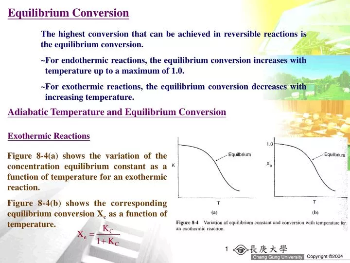
1. Equilibrium Conversion The highest conversion that can be achieved in reversible reactions is the equilibrium conversion. ~For endothermic reactions, the equilibrium conversion increases with temperature up to a maximum of 1.0. ~For exothermic reactions, the equilibrium conversion decreases with increasing temperature. Adiabatic Temperature and Equilibrium Conversion Exothermic Reactions Figure 8-4(a) shows the variation of the concentration equilibrium constant as a function of temperature for an exothermic reaction. Figure 8-4(b) shows the corresponding equilibrium conversion Xe as a function of temperature.

2. To determine the maximum conversion that can be achieved in an exothermic reaction carried out adiabatically, we find the intersection of the equilibrium conversion as a function of temperature with temperature-conversion relationships from the energy balance as shown in Figure 8-5. If the entering temperature is increased from T0 to T01, the energy balance line will be shifted to the right and will be parallel to the original line, as shown by the dashed line. Note that as the inlet temperature increases, the adiabatic equilibrium conversion decreases.

3. Example 8-6 For the elementary solid-catalyzed liquid-phase reaction make a plot of equilibrium conversion as a function of temperature. Determine the adiabatic equilibrium temperature and conversion when pure A is fed to the reactor at a temperature of 300 K. Solution Equilibrium Rate Law Stoichiometry (liquid phase, v=v0)

4. Equilibrium Constant Equilibrium Conversion from Thermodynamics

6. Reactor Staging with Interstate Cooling of Heating Higher conversions than those shown in Figure E8-6.1 can be achieved for adiabatic operation by connecting reactors in series with interstage cooling: The conversion-temperature plot for this scheme is shown in Figure 8-6. We see that with three interstage coolers 90% conversion can be achieved compared to an equilibrium conversion of 40% for no interstage cooling.

7. Endothermic Reactions The first reaction step (k1) is slow compared to the second step, and each step is highly endothermic. The allowable temperature range for which this reaction can be carried out is quite narrow: Above 530C undesirable side reactions occur, and below 430C the reaction virtually does not take place. A typical feed stock might consist of 75% straight chains, 15% naphthas, and 10% aromatics. Note that the reactors are not all the same size. Typical sizes are on the order of 10 to 20 m high and 2 to 5 m in diameter. Because the reaction is endothermic, equilibrium conversion increases with increasing temperature. A typical equilibrium curve and temperature conversion trajectory for the reactor sequence are shown in Figure 8-8.

8. Example 8-7 What conversion could be achieved in Example 8-6 if two interstage coolers that had the capacity to cool the exit stream to 350 K were available? Also determine the heat duty of each exchanger for a molar feed rate of A of 40 mol/s. Assume that 95% of equilibrium conversion is achieved in each reactor. The feed temperature to the first reactor is 300 K. Solution 1. Calculate Exit Temperature We now cool the gas stream exiting the reactor at 460 K down to 350 K in a heat exchanger.

9. 2. Calculate the Heat Load no reaction in the exchanger 220 kcal/s must be removed to cool the reacting mixture from 460 K to 350 K for a feed rate of 40 mol/s 3. Calculate the Coolant Flow Rate

10. 4. Calculate the Heat Exchange Area 5. Second Reactor

11. Optimum Feed Temperature Consider an adiabatic reactor of fixed size or catalyst weight and investigate what happens as the feed temperature is varied. The reaction is reversible and exothermic. At one extreme, using a very high feed temperature, the specific reaction rate will be large and the reaction will proceed rapidly, but the equilibrium conversion will be close to zero. As a result, very little product will be formed. At the other extreme of low feed temperatures, little product will be formed because the reaction rate is so low. A plot of the equilibrium conversion and the conversion calculated from the adiabatic energy balance, is shown in Figure 8-9. We see that for an entering temperature of 600 K the adiabatic equilibrium conversion is 0.15. The corresponding conversion profiles down the length of the reactor are shown in Figure 8-10. The equilibrium conversion also varies along the length of the reactor as shown by the dashed line in Figure 8-10. We also see that at the high entering temperature, the rate is very rapid and equilibrium is achieved very near the reactor entrance.

12. We notice that the conversion and temperature increase very rapidly over a short distance (i.e., a small amount of catalyst). This sharp increase is sometime referred to as the “point” or temperature at which the reaction ignites. If the inlet temperature were lowered to 500 K, the corresponding equilibrium conversion is increased to 0.38; however, the reaction rate is slower at this lower temperature so that this conversion is not achieved until closer to the end of the reactor. If the entering temperature were lowered further to 350 K, the corresponding equilibrium conversion is 0.75, but the rate is so slow that a conversion of 0.05 is achieved for the specified catalyst weight in the reactor. At a very low feed temperature, the specific reaction rate will be so small that virtually all of the reactant will pass through the reactor without reacting. It is apparent that with conversions close to zero for both high and low feed temperatures there must be an optimum feed temperature that maximizes conversion. As the feed temperature is increased from a very low value, the specific reaction rate will increase, as will the conversion. The conversion will continue to increase with increasing feed temperature until the equilibrium conversion is approached in the reaction. Further increases in feed temperature for this exothermic reaction will only decrease the conversion due to the decreasing equilibrium conversion. This optimum inlet temperature is shown in Figure 8-11.

13. CSTR with Heat Effects Although the CSTR is well mixed and the temperature is uniform throughout the reaction vessel, these conditions do not mean that the reaction is carried out isothermally. Isothermal operation occurs when the feed temperature is identical to the temperature of the fluid inside the CSTR. The rate of heat transfer from the exchanger to the reactor is For exothermic reactions, T>Ta2>Ta1 For endothermic reactions, Ta1>Ta2>T

14. An energy balance on the coolant fluid entering and leaving the exchanger is Assuming a quasi-steady for the coolant flow and neglecting the accumulation term (i.e., dTa/dt=0) Cpc is the heat capacity of the coolant fluid TR is the reference temperature. for large coolant flow rates

17. Example 8-8 Propylene glycol is produced by the hydrolysis of propylene oxide: Over 800 million pounds of propylene glycol were produced in 2004 and the selling price was approximately $0.68 per pound. Propylene glycol makes up about 25% of the major derivatives of propylene oxide. The reaction takes place readily at room temperature when catalyzed by sulfuric acid. You are the engineer in charge of an adiabatic CSTR producing propylene glycol by this method. Unfortunately, the reactor is beginning to leak, and you must replace it. (You told your boss several times that sulfuric acid was corrosive and that mild steel was a poor material for construction.) There is a nice-looking overflow CSTR of 300-gal capacity standing idle; it is glass-lined, and you would like to use it. You are feeding 2500 lb/h (43.04 lb mol/h) of propylene oxide (P.O.) to the reactor. The feed stream consists of (1) an equivolumetric mixture of propylene oxide (46.62 ft3/h) and methanol (46.62 ft3/h), and (2) water containing 0.1 wt% H2SO4. The volumetric flow rate of water is 233.1 ft3/h, which is 2.5 times the methanol-P.O. flow rate. The corresponding molar feed rates of methanol and water 71.87 and 802.8 lb mol/h, respectively. The water-propylene-oxide-methanol mixture undergoes a slight decrease in volume upon mixing (approximately 3%), but you neglect this decrease in your calculations. The temperature of both feed streams is 58F prior to mixing, but there is immediate 17F temperature rise upon mixing of the two feed streams caused by the heat of mixing. The entering temperature of all feed streams is thus taken to be 75F (Figure E8-8.1).

18. Furusawa et. al. state that under conditions similar to those at which you are operating, the reaction is first-order in propylene oxide concentration and apparent zero-order in excess of water with the specific reaction rate The units of E are Btu/lb mol. There is an important constraint on your operation. Propylene oxide is a rather low-boiling substance. With the mixture you are using, you feel that you can not exceed an operating temperature of 125F, or you will lose too much oxide by vaporization through the vent system. Can you use the idle CSTR as a replacement for the leaking one if it will be operated adiabatically? If so, what will be the conversion of oxide to glycol?

19. Solution In this problem, neither the exit conversion nor the temperature of the adiabatic reactor is given. By application of the material and energy balances we can solve two equation with two unknowns (X and T). Solving these coupled equations we determine the exit concentration and temperature for the glass-lined reactor to see if it can be used to replace the present reactor. 1. Mole Balance (design equation) 4. Combining 2. Rate Law 3. Stoichiometry (liquid phase)

20. 5. Energy Balance 6. Calculations a. Heat of reaction at temperature T b. Stoichiometry

21. c. Evaluate mole balance terms d. Evaluate energy balance terms

22. X=0.85 T=613R We observe from this plot that the only intersection point is at 85% conversion and 613R. At this point, both the energy balance and mole balance are satisfied. Because the temperature must remain below 125F (585R), we cannot use the 300-gal reactor as it is now.

23. Example 8-9 A cooling coil has been located in equipment storage for use in the hydration of propylene oxide discussed in Example 8-8. The cooling coil has 40 ft2 of cooling surface and the cooling water flow rate inside the coil is sufficiently large that a constant coolant temperature of 85F can be maintained. A typical overall heat-transfer coefficient for such a coil is 100 Btu/hft2F. Will the reactor satisfy the previous constraint of 125F maximum temperature if the cooling coil is used? Solution

24. X=0.36 T=564R

25. Multiple Steady States Consider the steady-state operation of a CSTR in which a first-order reaction is taking place. heat-generated term heat-removed term

26. Heat-Removed Term, R(T) We see that R(T) increases linearly with temperature, with slope CP0(1+). As the entering temperature T0 is increased, the line retains the same slope but shifts to the right as shown in Figure 8-14. If one increase  by either decreasing the molar flow rate FA0 or increasing the heat-exchange area, the slope increases and the ordinate intercept moves to the left as shown in Figure 8-15, for conditions of Ta<T0. Note that if Ta>To, the intercept will move to the right as  increases.

27. Heat-Generated Term, G(T) first-order liquid reaction second-order liquid reaction Low E high E low T high T

28. Ignition-Extinction Curve As the entering temperature is increased, the steady-state temperature increases along the bottom line until T05 is reached. Any fraction of a degree increase in temperature beyond T05 and the steady-state reactor temperature will jump up to Ts11, as shown in Figure 8-20. The temperature at which this jump occurs is called the ignition temperature. If a reactor were operating at Ts12, and we began to cool the entering temperature down from T06, the steady-state reactor temperature Ts3 would eventually be reached, corresponding to an entering temperature T02. Any slight decrease below T02 would drop the steady-state reactor temperature to Ts2. As a result, T02 is called the extinction temperature.

29. Ts8 Ts9 G>R T unstable steady state Ts8 Ts8 Ts7 R>G T Ts9 Ts9 R>G T Ts9 Ts9 Ts9 G>R T locally stable Ts7 Ts7 R>G T Ts7 Ts7 Ts7 G>R T

30. in a CSTR operated adiabatically The multiple steady-state temperatures were examined by varying the flow rate over a range of space times, , as shown in Figure 8-23. One observes from this figure that at a space-time of 12 s, steady-state reaction temperatures of 4, 33, and 80C are possible. If one were operating on the higher steady-state temperature line and the volumetric flow rates were steadily increase (i.e., the space-time decreased), one notes that if the space velocity dropped below about 7 s, the reaction temperature would drop from 70C to 2C. The flow rate at which this drop occurs is referred to as the blowout velocity.

31. Runaway Reactions in a CSTR For a CSTR, we shall consider runway (ignition) to occur when we move from the lower steady state to the upper steady state. The ignition temperature occurs at the point of tangency of the heat removed curve to the heat-generated curve. If we move slightly off this point of tangency as shown in Figure 8-24, then runway is said to have occurred. For the heat-removed curve, the slope is For the heat-generated curve, the slope is

32. If this difference between the reactor temperature and Tc, Trc, is exceeded, transition to the upper steady state will occur. For many industrial reactions E/RT is typically between 16 and 24, and the reaction temperatures may be between 300 to 500 K. As a result, this critical temperature difference Trc will be somewhere around 15 to 30C.

33. From Figure 8-25, we see that for a given value of [CP0(1+)], if we were to increase the entering temperature T0 from some low-value T01 (Tc1) to a higher entering temperature value T02 (Tc2), we would reach a point at which runway would occur.

34. Nonisothermal Multiple Chemical Reactions Energy Balance for Multiple Reactions in Plug-Flow Reactors q multiple reactions m species Consider the following reaction sequence carried out in a PFR:

35. Example 8-10 The following gas-phase reaction occur in a PFR: Pure A is fed at a rate of 100 mol/s, a temperature of 150C, and a concentration of 0.1 mol/dm3. Determine the temperature and flow rate profiles down the reactor.

36. Solution Rate Law Mole Balance Relative Rates Net Rates

37. Stoichiometry (gas phase P=0) Energy Balance

38. FA=0

39. Energy Balance for Multiple Reactions in CSTR q multiple reactions m species For two parallel reactions,

40. Example 8-11 The elementary liquid-phase reactions take place in a 10-dm3 CSTR. What are the effluent concentrations for a volumetric feed rate of 1000 dm3/min at a concentration of A of 0.3 mol/dm3? The inlet temperature is 283 K.

41. Solution The reactions follow elementary rate laws Mole Balance on Every Species Rate Law

42. Energy Balance

44. Closure ~Virtually all reactions that are carried out in industry involve heat effects. This section provides the basis to design reactors that operate at steady state and involve heat effects. ~To model these reactors, we simply add another step to our algorithm; this step is the energy balance. Here it is important to understand how the energy balance was applied to each reaction type so that you will be able to describe what would happen if you changed some of the operating conditions (e.g., T0). ~Another major goal after studying this section is to able to design reactors that have multiple reactions taking place under nonisothermal conditions.