Download
1 / 79
860 likes | 1.18k Vues
Phylogeny. Definition and Assumptions Input data for computing phylogenies Character-based Approaches Distance-based Approaches. Phylogeny. Definition and Assumptions Input data for computing phylogenies Character-based Approaches Distance-based Approaches. Definition. Assumption

E N D
Phylogeny • Definition and Assumptions • Input data for computing phylogenies • Character-based Approaches • Distance-based Approaches
Phylogeny • Definition and Assumptions • Input data for computing phylogenies • Character-based Approaches • Distance-based Approaches
Definition • Assumption • All organisms on Earth have a common ancestor • This implies that any set of species is related. • Phylogeny • The relationship between any set of species. • Phylogenetic tree • Usually, the relationship can be represented by a tree which is called a phylogenetic tree • this is not always true
Example Time giant panda moose lesser panda duck goshawk vulture alligator
(Input) Sequence Data (Last week) Align Sequences (Skip) Assess phylogenetic signal (Assumptions) Choose character or distance approach (Assumptions) Choose distance measure Choose optimality criterion (Assumptions) Choose algorithm (Skip) Test reliability Phylogenetic Inference Apply algorithm to calculate tree(s) Based loosely on paper from Hillis, Allard, and Miyamoto 1993
Comments • Most work focuses on binary or bifurcating trees • Nodes correspond to organisms at a bifurcation or splitting event • Edges represent time/evolutionary distance between the ancestor/descendant nodes • Existing organisms are always placed at the leaves • The organisms corresponding to an internal node may be identical to an organism at a leaf
What algorithms do • Root location • Some algorithms attempt to recreate the topology of the tree with a root • Many create unrooted topologies • Edge lengths • Some algorithms attempt to estimate edge lengths (evolutionary divergence) • Others focus only on topology
Key Point • Almost every step of the process involves assumptions • It is important to understand these assumptions • I’ll try to highlight some of them along with the main algorithmic ideas
Phylogeny • Definition and Motivation • Input data for computing phylogenies • Character-based Approaches • Distance-based Approaches
Input Data • Two main types • Distance data • Estimate of “distance” between all pairs of organisms • “Character” data • A set of features with a defined set of feature values • A feature value for each organism
Distance Data • Distances ideally should reflect the amount of time between when organisms had a common ancestor • This is typically not true • We’ll talk more about distance data when we get to algorithms that work with distance data
Character Data • Historically • morphological (form and structure) data • e.g., vertebrate versus invertebrate • Currently • Gene sequence data • DNA sequence of a gene • Amino acid sequence of a specific protein • Rarely an entire genome
Alignments and Sequence Data • When working with sequence data, current techniques ignore order • One sequence per organism • Perform a multiple sequence alignment • Each position is now treated independently of others • In many cases, screening is performed to select “most informative” positions
Phylogeny • Definition and Motivation • Input data for computing phylogenies • Character-based Approaches • Maximum Parsimony definition • Heuristics • Upper bound on maximum parsimony • Maximum likelihood • Distance-based Approaches
Maximum Parsimony • Assumption • We have correctly aligned sequence data, so we don’t have to worry about insertions/deletions • Goal • Find a phylogenetic tree that explains the observed sequences with a minimal number of substitutions
Aligned input AAAG AAAC AGGG AGGT Screened input Position 1 is identical in all organisms AAG AAC GGG GGT Example
GGG (2) AAG AAG (2) (2) GGG GGG AAG AAG (1) (3) (1) (3) GGG AAC GGT AAG Possible trees GGG GGT AAC AAG
Brute Force Algorithm • Generate all possible trees for the given number of organisms • Suppose there are n taxa. • How many binary rooted trees are possible? • How many binary unrooted trees are possible? • For each possible tree, consider all possible assignments of the n taxa to the leaves of the tree • How many possible assignments are there? • For each tree and assignment, calculate best possible assignment of characters to the internal nodes of the tree and calculate resulting score • Each position can be calculated independently • Save most best scoring trees (and potentially assignments)
Computing cost • Treat each character independently • Bottom up processing • post-order traversal of the tree • Data needed • At each node v, store a set of possible values R(v) such that any one of these would be minimal cost • Global variable C for cost initialized to 0
Computing internal nodes and cost • At leaf node v: R(v) = the value of the taxa at v • Internal node v with children w and x: • If R(w) intersect R(x) is not empty, R(v) = R(w) intersect R(x) • Otherwise, R(v) = R(w) union R(x) and increment C by 1 • Traceback: • At root r, choose any value in R(r) • At node v, choose value at parent if in R(v). Else choose anything
Example C = 0 B A B A
Example C = 1 B {A,B} A B A
Example C = 1 {A} B {A,B} A B A
Example {A,B} C = 2 {A} B {A,B} A B A
Example B (1) C = 2 {A} B {A,B} A B A
Example B (1) C = 2 A B {A,B} A B A
Example B (1) C = 2 A B A A (1) B A
Running time • Brute force • (Number of trees) * (Number of assignments) * (cost to compute internal nodes) • Very large • Is there a better algorithm? • Yes, but the problem is NP-hard • This means that the best known solution for computing a phylogenetic tree of n taxa has a worst-case running time that is not polynomial in n • In practice, this means computing the optimal phylogenetic tree is extremely time-consuming for relatively small numbers of taxa • (17 was limit according to a paper in 1997)
Comments • Weighted parsimony • The basic approach can be extended to allow for non-equal substitution probabilities • For example, replacing an A with a G may be more or less costly than replacing an A with a T • Basic procedure outline is the same, but now we must consider all possible character values at each internal node • Root of tree • We can search for unrooted trees as root values will be identical to one of its children in all cases (assuming triangle inequality on costs in the weighted parsimony case)
Heuristics • Heuristics with non-optimal guarantees • Stochastic local search • Start with a tree and an assignment • Stochastically search through space of all possible trees by making local changes and retaining value if there is improvement • Incremental addition of taxa • Start with tree for any three taxa • Incrementally add a new taxa at best possible edge • Different orderings lead to different final trees • Branch and bound • Search through all possible trees and assignments but keep track of current best and eliminate possibilities as they provably cannot be optimal
Upper bound on parsimony • Assumption • Triangle inequality in scoring function • S(i,j) + S(j,k) >= S(i,k) • Definition • Given a set of species S • Let G(S) be the weighted complete graph • nodes represent species in S • edges represent distance between two species • Theorem • Any minimum spanning tree on G(S) has total length at most twice that of the most parsimonious tree of the species in T • Minimum weight spanning trees can be computed efficiently
Proof Suppose the above is a most parsimonious tree T* for the set of species represented by the green nodes at the leaves
Double edges on graph Parsimony weight is now twice optimal value
Create Eulerian Tour 1 14 15 20 2 7 8 13 3 4 5 6 9 10 11 12 16 17 18 19 Eulerian tour traverses each edge exactly once and is guaranteed to exist once we double edges. Cost of traversing all edges is exactly twice that of optimal tree T*
Focus on green nodes 1 14 15 20 2 7 8 13 3 4 5 6 9 10 11 12 16 17 18 19 A B C D E F A to B: Edges 4-5 B to C: Edges 6-9 C to D: Edges 10-11 D to E: Edges 12-16 E to F: Edges 17-18 F to A: Edges 19-20 and 1-3
A B C D E F Tour in graph G(S) 1 14 15 20 2 7 8 13 3 4 5 6 9 10 11 12 16 17 18 19 A B C D E F S(A,B) <= distance on edge 4 + distance on edge 5
Final result 1 14 15 20 2 7 8 13 3 4 5 6 9 10 11 12 16 17 18 19 A B C D E F A B C D E F Weight of all edges on path <= twice weight of T*. This path is one possible spanning tree of G(S). Therefore, result follows.
Comments about Parsimony • Assumptions • Sequence data has limited homoplasy • Substitution scheme encodes assumptions about evolutionary process • (example: 3rd codon substitution frequencies higher than at other positions) • Minimum number of changes is best explanation • Other comments • There are probabilistic models where parsimony will converge on the wrong tree even given infinite data • Differing rates of evolution in different parts of the tree can cause problems
Maximum Likelihood • Assumption • We have correctly aligned sequence data, so we don’t have to worry about insertions/deletions • We have a model of evolution • Goal • Find a phylogenetic tree that would have the highest probability (subject to our model of evolution) of generating the observed sequences
Formalizing max likelihood • We want to find a phylogenetic tree that maximizes P(data | tree) • Data • set of n aligned sequences s = s1, s2, …, sn • Tree • Topology T with n leaves • set of edges lengths t = t1, t2, …, t2n-2 • There are 2n-2 edges in a rooted binary tree with n leaves • We want to find (T, t) such that P(s | (T, t)) is maximized
x7 t5 t6 x5 x6 t1 t2 t3 t4 s1 s2 s3 s4 Example • Let P(x | y, t) denote the probability that ancestral sequence y evolves into sequence s along an edge of length t • Assume t is proportional to mutation rate * evolutionary time • P(s | (T,t)) = sum over all x5, x6, x7 • p(x7) P(x5|x7,t5) P(x6|x7,t6) P(s1|x5,t1) P(s2|x5,t2) P(s3|x6,t3) P(s4|x6,t4)
Models of Evolution • What should P(x|y, t) be? • Two assumptions of commonly used models • Each site evolves independently • There are only substitutions, no insertions/deletions • P(x|y, t) = Pi=1 to m P(x(i) | y(i), t) • m is sequence length
A C G T rt = 1/4 (1 + 3e-4at) st = 1/4 (1 - e-4at) Limit values when t = 0 or t = infinity? rt st st st A st rt st st C G st st rt st T st st st rt Jukes-Cantor Model [1969] • What should P(x(i)|y(i), t) be? • Jukes-Cantor Model [1969] • parameter a
A C G T st = 1/4 (1 - e-4bt) ut = 1/4 (1 + e-4bt -2e-2(a+b)t) rt = 1 - 2st - ut Limit values when t = 0 or t = infinity? rt st ut st A st rt st ut C G ut st rt st T st ut st rt Kimura Model [1980] • What should P(x(i)|y(i), t) be? • Kimura Model [1980] • parameters a, b
Properties of Models of Evolution • Assumptions • Substitution process is Markovian and stationary • probabilities do not change over time • length of time interval is all that matters • Substitution matrix is multiplicative • Matrix(t) * Matrix (s) = Matrix (t+s) • Sb P(a|b, t)P(b|c, s) = P(a|c, s+t)
Computing Likelihood • P(Lv|a) = probability of all leaves below node v having their values given the residue at node v is a • Recursive algorithm for computing P(Lv|a) • Base Case: v is a leaf node • P(Lv|a) = 1 if a is the value of residue at that leaf, 0 otherwise • Recursive case: v is an internal node • Compute P(Lu|x), P(Lw|x) for all x at daughter nodes v and w • 2 |S| values total • Set P(Lv|a) = Sx,y P(x|a, tu)P(Lu|x) P(y|a, tw)P(Lw|y) • |S|2 distinct products to compute
Brute Force Algorithm • Generate all possible topologies for the given number of organisms • For each possible tree, consider all possible assignments of the n taxa to the leaves of the tree • Compute likelihood of tree topology generating data • For each tree and assignment, consider all possible interior tree node assignments • Generate likelihood for topology as a function of edge length variables • Solve equations to determine best edge lengths for given topology • Save the tree that has the resulting data with highest probability • More complex than computing maximum parsimony
Comments about Max Likelihood • Accuracy of tree is obviously highly dependent on the accuracy of the model of evolution that is assumed • If substitution matrices are multiplicative and a “reversibility” constraint holds, then max likelihood cannot predict position of root • Extremely slow in the general case for even relatively small numbers of taxa (depending on the model of evolution assumed)
Posterior distribution • Max likelihood: • Finds phylogenetic tree that maximizes P(data | tree) • Posterior distribution is even better: • Find phylogenetic tree such that maximizes P(tree | data) • Bayes Theorem • P(tree | data) = [P(data | tree) P(tree)] / P(data) • If we know prior distribution of P(tree), then we can do some sampling techniques to estimate posterior distribution P(tree | data) • There are ways to finesse not knowing P(data)
Phylogeny • Definition and Motivation • Input data for computing phylogenies • Character-based Approaches • Distance-based Approaches • Data assumptions • Molecular clock and ultrametric properties • Simple clustering algorithms • Additivity properties • Neighbor joining