Download
1 / 22
220 likes | 382 Vues
Predictions from the regression model. (Session 09). Learning Objectives. At the end of this session, you will be able to assess the regression model in terms of its appropriateness as a prediction equation distinguish between two types of possible predictions and why their precision differs

E N D
Predictions from the regression model (Session 09)
Learning Objectives At the end of this session, you will be able to • assess the regression model in terms of its appropriateness as a prediction equation • distinguish between two types of possible predictions and why their precision differs • use software to produce predictors and corresponding confidence intervals • understand dangers of predicting beyond values used in developing the predictor
An Example Consider a health survey of a random sample of 20 districts in which one variable of interest was the perinatal mortality rate, i.e. no. of deaths in first 30 days after birth per 1000 live births; In all districts, the number of health centres per 1000 households is known. Suppose a health official wants to predict perinatal mortality in districts not covered by the survey.
Results of a linear regression model ----------------------------------------- mort | Coef. Std.Err. t P>|t| ----------+------------------------------ hcentres | -1.9139 .4071 -4.70 0.000 const. | 38.111 4.703 8.10 0.000 ----------------------------------------- Adjusted R2 = 52.6% The equation of the line is: mort = 38.11 - 1.914 (hcentres)
Predictions from the model • There are two types of predictions possible: • What would be the average mortality rate in districts where there are only 9 health centres per 1000 households? • A particular district has 9 health centres per 1000 hhs. What would be the predicted mortality rate in this district? • The answer to both predictions are: • mortality = 38.11 - 1.914(9)= 20.88 • But would their standard errors be the same?
Standard errors of the predictions The standard error for (1), call it “sepred”, can be obtained with statistical software. The standard error for (2) is the square root of: (sepred)2 + (residual M.S. in anova) The addition of the RMS is to account for variation of individual values about their mean. Note: For the case where there is only 1 regressor variable, a simple formula does exist (see final slide).
Confidence intervals for predictions The standard error can be used to determine (say) 95% confidence intervals for each type of prediction. Because individual predictions have a larger standard error, the corresponding 95% C.I. will be wider for such predictions. The graphs below show the difference in precision (Stata output)
Dangers of extrapolation It is clear from above graphs that the confidence bands widen as predictions are made away from the mean of the x values. This is also true of predictions made from results of a multiple linear regression model. Hence extrapolating to make predictions beyond x’s used in the model fitting can be dangerous since they would be very imprecise!
A real example from Tanzania One aim of the Adult Morbidity and Mortality Project (AMMP) in Tanzania was to investigate how health outcomes varied across different levels of poverty. All households in several sentinel sites were monitored over many years… But, initially there was no measure of income poverty to address above objective. Question: Can a prediction model be developed to give a poverty measure using socio-economic variables?
Results for a model for households in Tabora region ------------------------------------------ lnexpdf | Coef. Std.Err. t P>|t| -------------+---------------------------- hhsize | -.22667 .01213 -18.69 0.000 hhsize2 | .00956 .00085 11.24 0.000 water | .11726 .03007 3.90 0.000 qmeat | .11932 .0100 11.93 0.000 qmilk | .03158 .00601 5.26 0.000 iron | .20931 .03164 6.62 0.000 table | .18927 .03559 5.32 0.000 wheatf | .29468 .03232 9.12 0.000 seeds | .18994 .05095 3.73 0.000 num_meal | .15502 .03265 4.75 0.000 const. | 9.1540 .0930 98.41 0.000 ------------------------------------------
Model equation lnexpdf (y) = 9.154 – 0.227(hhsize) + 0.0096(hhsize)2 + 0.117(water) + 0.119(qmeat) + 0.032(qmilk) + 0.209(iron) +0.189(table) + 0.295(wheatf) + 0.190(seeds) +0.155(num_meal)
How good is the prediction? R2=58%. A plot of predicted values vs actual also indicates closeness of prediction.
But terciles tabulation of actual versus predicted, less promising! terciles | terciles of prediction|of lnexpdf| Lowest Middle Highest | Total ----------+-------------------------+------ Lowest | 248 80 13 | 341 Middle | 95 182 74 | 351 Highest | 9 86 262 | 357 ----------+-------------------------+------ Total | 352 348 349 | 1049 ----------+-------------------------+------ Percent correctly classified = [(248 + 182 + 262)/1049]*100 = 66%
How many HHs are correctly classified as being below poverty line? ---------------+-------------------+------ If really below| Below poverty line| basic needs | on predictions | poverty line? | No Yes | Total ---------------+-------------------+------ No | 838 42 | 880 Yes | 99 70 | 169 ---------------+-------------------+------ Total | 937 112 | 1,049 ---------------+-------------------+------ Percent correctly classified as below line = [(838 + 70)/1049]*100 = 86.6%
Does the prediction address the original objective? The answer is “yes”. Although at a household level, the predictions were not so good, health outcomes like mortality rates, percent immunised, etc., were measured in AMMP at community level. The predictions, averaged over HHs in a community were satisfactory, e.g. further analysis showed that the average prediction percent error was under 6%.
Key Steps in model prediction… • Select carefully a set of potential explanatory variables • Decide the direction of influence expected (+ or – for regression coefficients) • Use a suitable model selection approach to identify the subset of variables contributing significantly to explaining the variation in the key response(y) • Conduct a residual analysis and take remedial action if problems occur
Key Steps in model prediction… • Check whether the final model makes sense in terms of the explanatory variables included and the signs of their coefficients • Consider whether there are other latent variables which may be non-measurable but influential! Conclusions should mention these! • Examine how well the prediction performs, studying also the precision of the prediction • Give the form of the model equation and corresponding conclusions
Formulae for standard errors for a simple linear regression(for reference only) If s2 represents the Residual Mean Square in the anova, the std. error for the predicted mean = Std. error for a predicted individual value =
Practical work follows to ensure learning objectives are achieved…