Download
1 / 49
490 likes | 616 Vues
Towards Simple, High-performance Input-Queued Switch Schedulers. Devavrat Shah Stanford University. Joint work with Paolo Giaccone and Balaji Prabhakar. Berkeley, Dec 5. Outline. Description of input-queued switches Scheduling the problem some history

E N D
Towards Simple, High-performance Input-Queued Switch Schedulers Devavrat Shah Stanford University Joint work with Paolo Giaccone and Balaji Prabhakar Berkeley, Dec 5
Outline • Description of input-queued switches • Scheduling • the problem • some history • Simple, high-performance schedulers • Laura • Serena • Apsara • Conclusions
The Input-Queued (IQ) Switch Architecture • N inputs, N outputs (in fig, N = 3) • Time is slotted • at most one packet can arrive per time-slot at each input • Equal sized cells/packets • Buffers only at inputs • Use a crossbar for switching packets
Scheduling • Crossbar is defined by these constraints: in each time-slot • only one packet can be transferred to each output • only one packet can be transferred from each input • The scheduling problem: Subject to the above constraint, find a matching of inputs and outputs • i.e. determine which output will receive a packet from which input in each time slot
Background to switch scheduling • [Karol et al. 1987] Throughput is limited due to head-of-line blocking (limited to 58% for Bernoulli IID uniform traffic) • [Tamir 1989] Observed that with “Virtual Output Queues” (VOQs) head-of-line blocking is eliminated.
Basic Switch Model S(t) L11(t) A11(t) 1 1 D1(t) A1N(t) AN1(t) DN(t) N N ANN(t) LNN(t)
Some definitions 3. Queue occupancies: Occupancy L11(t) LNN(t)
More background on theory [Anderson et al. 1993] A schedule is equivalent to finding a matching in a bipartite graph induced by input and output nodes
Background 20 3 2 30 25 [McKeown et al. 1995] (a) Maximum size match does not give 100% throughput.(b) But maximum weight match can, where weight can be queue-length, age of a cell 20 MWM 30 25
Maximum Weight Matching • Maximum weight matching (MWM) • 100% throughput • provable delay bounds for i.i.d. Bernoulli admissible traffic • but, finding MWM is like solving a network-flow problem whose complexity is -- complex for high-speed networks • We seek to approximate maximum weight matching • Our goal: • obtain a simply implementable approximation to MWM that performs competitively with MWM
Approximating MWM • Two performance measures • throughput • delay • We first consider simple approximations to MWM that deliver 100% throughput (i.e. stability), and then deal with delay
Methods of Approximation • Randomization • well-known method for simplifying implementation • Using information in packet arrivals • since queue-sizes grow due to arrivals, and arrival times are a source of randomness • Hardware parallelism • yields an efficient search procedure
Randomization • The main idea of randomized algorithms is • to simplify the decision-making process by basing decisions upon a small, randomly chosen sample from the state rather than upon the complete state
An Illustrative Example • Find the oldest person from a population of 1 billion • Deterministic algorithm: linear search • has a complexity of 1 billion • A randomized version: find the oldest of 30 randomly chosen people • has a complexity of 30 (ignoring complexity of random sampling) • Performance • linear search will find the absolute oldest person (rank = 1) • if R is the person found by randomized algorithm, we can make statements like P(R has rank < 100 million) > 0.95 • thus, we can say that the performance of the randomized algorithm is very good with a high probability
Randomizing Iterative Schemes • Often, we want to perform some operation iteratively • Example: find the oldest person each year • Say in 2001 you choose 30 people at random • and store the identity of the oldest person in memory • in 2002 you choose 29 new people at random • let R be the oldest person from these 29 + 1 = 30 people P(R has rank < 100 million) or, P(R has rank < 50 million)
Back to Switch Scheduling: Randomizing MWM • Choose d matchings at random and use the heaviest one as the schedule • Ideally we would like to have small d. However: • Theorem: Even with d = N this algorithm doesn’t yield 100% throughput!
Simulation Scenario • Switch Size : 32 X 32 • Input Traffic (shown for a 4 X 4 switch) • Bernoulli i.i.d. inputs • diagonal load matrix: • normalized load=x+y<1 • x=2y
Crucial Observation • The state of the switch changes due to arrivals & departures • Between consecutive time slots, a queue’s length can change at most by 1 • hence a heavy matching tends to stay heavy • Therefore • ‘’remembering’’ a heavy matching should help in improving the performance
Tassiulas’ Algorithm • [Tassiulas 1998] proposed the following algorithm based on this observation: • let S(t-1) be the matching used at time t-1 • let R(t) be a matching chosen uniformly at random • and let S(t) be the heavier of R(t) and S(t-1) • This gives 100% throughput ! • note the boost in throughput is due to the use of memory • But, delays are very large
Derandomization • Let G be a fully-connected graph where each node is one of the N! possible schedules • Construct a Hamiltonian walk, H(t), on G • H(t) cycles through the nodes of G • At any time t • let R(t) = H(t mod N!) • and let S(t) be the heavier of R(t) and S(t-1) • this also has 100% throughput, but delays are large (derandomization will be useful later)
Stability • Lemma: Consider IQ switch with Bernoulli i.i.d. inputs. Let B be a matching algorithm which ensures WB(t) >= W*(t) – c for every t. Then B is stable. • Theorem: WDER(t) >= W*(t) – 2N.N! Therefore, it is stable.
Delay • These simple approximations of MWM yield 100% throughput, but delays are large • To obtain good delays we’ll present three different algorithms which use the following features: • selective remembrance -- Laura • information in the arrivals -- Serena • hardware parallelism -- Apsara
Laura S(t-1) R(t) COMP Next time S(t) Tassiulas • COMP = Maximum • R(t) – uniform sample Laura • COMP = Merge, picks the best edges of two matchings • R(t) – non-uniform sample
Merging Procedure 10 50 10 40 30 10 70 10 60 20 Merging S(t-1) R W(S(t-1))=160 W(R)=150 10 – 40+10 -30+10-50= - 90 70-10+60-20=100 S(t) W(S(t)) = 250
Throughput • Theorem: • LAURA is stable under any admissible Bernoulli i.i.d. input traffic.
Average Backlog via Simulation • Switch size: N = 32 • Length of VOQ: QMAX = 10000 • Comparison with • iSLIP, iLQF, MUCS, RPA and MWM
Simulation • Traffic Matrices • uniform • diagonal • sparse • logdiagonal
SERENA Serena • Since an increase in queue sizes is due to arrivals • And arrivals are a source of randomness • Use arrivals to generate random matching
Serena S(t-1) R(t) = matching generated using arrivals Merge Next time S(t)
Merging Procedure 23 89 89 3 3 2 1 5 5 Merging R 23 W(R)=121 89 3 31 97 S(t) W(S(t))=243 23 7 47 11 31 97 S(t-1) Arr-R W(S(t-1))=209
Throughput Theorem: • SERENA achieves 100% throughput under any admissible i.i.d. Bernoulli traffic pattern
Apsara • One way to obtain MWM is to search the space of all N! matchings • A natural approximation: If S(t-1) is the current matching, then S(t) is the heaviest matching in a “neighborhood” of S(t-1) • It turns out that there is a convenient way of defining neighbors (both for theory and for practice)
Neighbors S(t) Example: 3 x 3 switch Neighbors Neighbors differ from S(t) in ONLY TWO edges (for all values of N)
Apsara Neighbors generated in parallel Hamiltonian Walk N1 N2 Nk H(t) S(t-1) MAX Next time S(t)
Apsara: Throughput • Theorem: Apsara is stable under any admissible i.i.d. Bernoulli traffic. (stability due to Hamiltonian matching) • Also, note that W(S(t)) >= W(S(t-1),t) • Theorem: If W(S(t)) = W(S(t-1),t) then W(S(t)) >= 0.5 W *(t) (this is not enough to ensure stability)
Limited Parallelism • The Apsara algorithm searches over neighbors in parallel • If space is limited to modules, then search over randomly chosen subsetof size K from all neighbors • And there are other (good) deterministic ways of searching a smaller neighborhood of matchings
Conclusions • We have presented novel scheduling algorithms for input-queued switches • Laura • Serena • Apsara • They are simple to implement and perform competitively with respect to the Maximum Weight Matching algorithm
References • L. Tassiulas, “Linear complexity algorithms for maximum throughput in radio networks and input-queued switches,” Proc. INFOCOM 1998. • D. Shah, P. Giaccone and B. Prabhakar, “An efficient randomized algorithm for input-queued switch scheduling,” Proc. of Hot Interconnects, 2001. • P. Giaccone, D. Shah and B. Prabhakar,” An Implementable Parallel Scheduler for Input-Queued Switches”, Proc. of Hot Interconnects, 2001. • P. Giaccone, B. Prabhakar and D. Shah, “Towards simple and efficient scheduler for high-aggregate IQ switches”, Submitted INFOCOM’02. • R. Motwani and P. Raghavan, Randomized Algorithms, Cambridge University Press, 1995.