Download
1 / 21
240 likes | 420 Vues
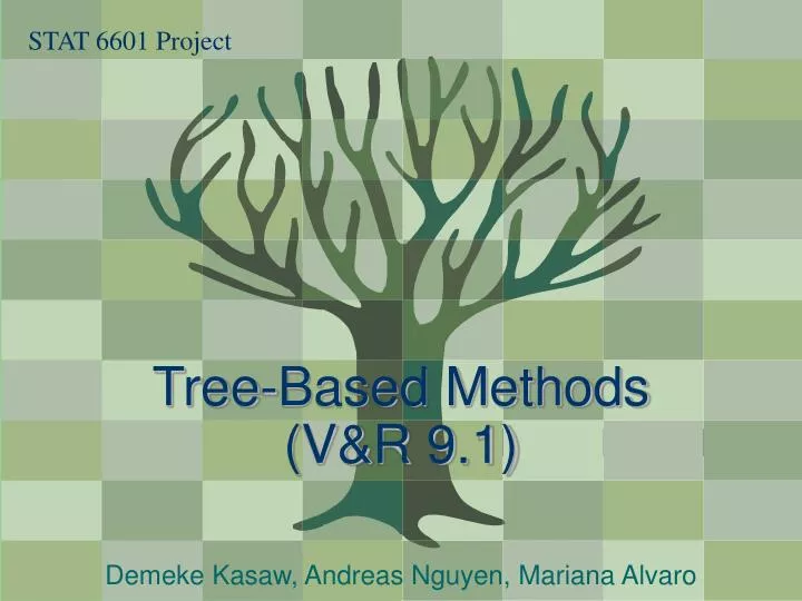
STAT 6601 Project. Tree-Based Methods (V&R 9.1). Demeke Kasaw, Andreas Nguyen, Mariana Alvaro. What are they? How do they work? Examples… Tree pictorials common. Simple way to depict relationships in data

E N D
STAT 6601 Project Tree-Based Methods(V&R 9.1) Demeke Kasaw, Andreas Nguyen, Mariana Alvaro
What are they? How do they work? Examples… Tree pictorials common. Simple way to depict relationships in data Tree-based methods use this pictorial to represent relationships between random variables. Overview of Tree-based Methods
Last Eruption < 3.0 min | Last Eruption < 4 .1 min 54.49 76.83 81.18 Trees can be used for bothClassification and Regression Time to Next Eruption vs. Length of Last Eruption Presence of Surgery Complications vs. Patient Age and Treatment Start Date | Start >= 8.5 months Start < 8.5 Present Start >= 14.5 Start < 14.5 Absent Age < 12 yrs Age >= 12 yrs Absent Sex = M Sex = F Absent Present
General Computation Issues and Unique Solutions • Over-Fitting: When do we stop splitting? Stop generating new nodes when subsequent splits only result in little improvement. • Evaluate the quality of the prediction: Prune the tree to ideally select the simplest most accurate solution. Methods: • Crossvalidation: Apply the tree computed from one set of observations (learning sample) to another completely independent set of observations (testing sample). • V-fold crossvalidation: Repeat the analysis with different randomly drawn samples from the data. Use the tree that shows the best average accuracy for cross-validated predicted classifications or predicted values.
Computational Details • Specify the criteria for predictive accuracy • Minimum costs: Lowest misclassification rate • Case weights • Selecting Splits • Define a measure of impurity for a node. A node is “pure” if they contain observations of a single class. • Determine when to stop splitting • All nodes are pure or contain no more than a n cases • Until all nodes contain no more than a specified Fraction of Objects • Selecting the “right-size” tree • Test sample cross validation • V Fold cross validation • Tree selection after pruning: if there are several trees with costs close to minimum, select the smallest-sized (least complex)
Computational Formulas • Estimation of Accuracy in Classification Trees • Resubstitution estimate • d(x) is the classifier • X=1 if X(d(xn) = jn) is true • X =0 if X(d(xn) = jn) is false • Estimation of Accuracy in Regression Trees • Resubstitution estimate
Computational FormulasEstimation of Node Impurity • Gini Index • Reaches zero when only one class is present at a node • P(j/t): probability of category j at node t • Entropy or Information
Classification Tree Example:What species are these flowers? Petal Length Petal Width Setosa tree Versicolor Sepal Length Sepal Width Virginica
Iris Classification Data • Iris dataset relates species to petal and sepal dimensions reported in centimeters. Originally used by R.A. Fisher and E. Anderson for a discriminant analysis example. • Data is pre-packaged in R dataset library and is available on DASYL. Sepal.Length Sepal.Width Petal.Length Petal.Width Species 6.7 3.0 5.0 1.7 versicolor 5.8 2.7 3.9 1.2 versicolor 7.3 2.9 6.3 1.8 virginica 5.2 4.1 1.5 0.1 setosa 4.4 3.2 1.3 0.2 setosa
Iris ClassificationMethod and Code library(rpart) # Load tree fitting packagedata(iris) # Load iris data # Let x = tree object fitting Species vs. all other# variables in iris with 10-fold cross validationx = rpart(Species~.,iris,xval=10) # Plot tree diagram with uniform spacing,# diagonal branches, a 10% margin, and a titleplot(x, uniform=T, branch=0, margin=0.1, main="Classification Tree\nIris Species by Petal and Sepal Length") # Add labels to tree with final counts,# fancy shapes, and blue text colortext(x,use.n=T,fancy=T,col="blue")
Classification Tree Iris Species by Petal and Sepal Length Petal.Length < 2 .45 Petal.Length >= 2 .45 setosa 50/0/0 Petal.Width < 1 .75 Petal.Width >= 1 .75 virginica versicolor 0/1/45 0/49/5 Results:
Identify this flower… Sepal Length 6 Sepal Width 3.4 Petal Length 4.5 Petal Width 1.6 Tree-based approach much simpler than the alternative Classification with Cross-validation True Group Put into Group setosa versicolor virginica setosa 50 0 0 versicolor 0 48 1 virginica 0 2 49 Total N 50 50 50 N correct 50 48 49 Proportion 1.000 0.960 0.980 N = 150 N Correct = 147 Linear Discriminant Function for Groups setosa versicolor virginica Constant -85.21 -71.75 -103.27 Sepal.Length 23.54 15.70 12.45 Sepal.Width 23.59 7.07 3.69 Petal.Length -16.43 5.21 12.77 Petal.Width -17.40 6.43 21.08 Classification Tree Iris Species by Petal and Sepal Length Setosa -85+24*6+24*3.4-16*4.5-17*1.6=41 Versicolor -72+16*6+7*3.4+5*4.5+6*1.6=80 PetalLength< 2 .45 PetalLength>= 2 .45 Virginica -103+12*6+4*3.4+13*4.5+21*1.6=75 Since Versicolor has highest score, we classify this flower as an Iris versicolor. setosa 50/0/0 PetalWidth>= 1 .75 PetalWidth< 1 .75 versicolor virginica 0/49/5 0/1/45
Regression Tree Example • Software used : R, rpart package • Goal: • Applying the regression tree method on CPU data, and predicting the response variable, ‘performance’.
CPU Data • CPU performance of 209 different processors. name syct mmin mmax cach chmin chmax perf 1 ADVISOR 32/60 125 256 6000 256 16 128 198 2 AMDAHL 470V/7 29 8000 32000 32 8 32 269 3 AMDAHL 470/7A 29 8000 32000 32 8 32 220 4 AMDAHL 470V/7B 29 8000 32000 32 8 32 172 5 AMDAHL 470V/7C 29 8000 16000 32 8 16 132 6 AMDAHL 470V/8 26 8000 32000 64 8 32 318 ... PerformanceBenchmark System Speed(mhz) Memory (kb) Cache (kb) Channels
R Code library(MASS); library(rpart); data(cpus); attach(cpus) # Fit regression tree to datacpus.rp <-rpart(log(perf)~.,cpus[,2:8],cp=0.001) # Print and plot complexity Parameter (cp) tableprintcp(cpus.rp); plotcp(cpus.rp) # Prune and display treecpus.rp<-prune(cpus.rp,cp=0.0055)plot(cpus.rp,uniform=T,main="Regression Tree")text(cpus.rp,digits=3) # Plot residual vs. predictedplot(predict(cpus.rp),resid(cpus.rp)); abline(h=0)
size of tree 1 3 5 7 11 14 17 1.2 1.0 0.8 X-val Relative Error 0.6 0.4 0.2 Inf 0.03 0.0072 0.0012 cp Determine the Best Complexity Parameter (cp) Value for the Model CP nsplit rel error xerror xstd 1 0.5492697 0 1.00000 1.00864 0.096838 2 0.0893390 1 0.45073 0.47473 0.048229 3 0.0876332 2 0.36139 0.46518 0.046758 4 0.0328159 3 0.27376 0.33734 0.032876 5 0.0269220 4 0.24094 0.32043 0.031560 6 0.0185561 5 0.21402 0.30858 0.030180 7 0.0167992 6 0.19546 0.28526 0.028031 8 0.0157908 7 0.17866 0.27781 0.027608 9 0.0094604 9 0.14708 0.27231 0.028788 10 0.0054766 10 0.13762 0.25849 0.026970 11 0.0052307 11 0.13215 0.24654 0.026298 12 0.0043985 12 0.12692 0.24298 0.027173 13 0.0022883 13 0.12252 0.24396 0.027023 14 0.0022704 14 0.12023 0.24256 0.027062 15 0.0014131 15 0.11796 0.24351 0.027246 16 0.0010000 16 0.11655 0.24040 0.026926 Cross-Validated Error SD Cross-Validated Error ComplexityParameter # Splits 1 – R2
Regression TreeAfter Pruning cach< 27 | cach< 27 | mmax< 6100 mmax< 2.8e+04 mmax< 2.8e+04 mmax< 6100 syct>=360 mmax< 1750 cach< 96.5 cach< 56 syct>=360 mmax< 1750 cach< 96.5 cach< 56 mmax< 2500 chmin< 5.5 mmax< 1.124e+04 2.51 2.95 5.35 5.22 6.14 chmax< 4.5 cach< 0.5 chmax< 14 5.22 6.14 chmin< 5.5 3.05 4.55 4.21 2.51 3.29 mmax< 1.1e+04 syct< 110 chmin>=1.5 2.95 5.35 3.12 3.52 4.69 5.14 cach< 0.5 mmax< 1.4e+04 3.26 3.54 3.89 4.55 4.21 4.92 4.04 4.31 3.52 4.03 Regression Tree Regression TreeBefore Pruning
How well does it fit? • Plot of residuals
Summary • Advantages of C & RT • Simplicity of results: • The interpretation of results summarized in a tree is very simple. • This simplicity is useful for purposes of rapid classification of new observations • It is much easier to evaluate just one or two logical conditions. • Tree methods are nonparametric and nonlinear • There is no implicit assumption that the underlying relationships between the predictor variables and the dependent variable are linear, follow some specific non-linear link function
References • Venables, Ripley (2002), Modern Applied Statistics with S,251-266. • StatSoft (2003) “Classification and Regression Trees”, Electronic Textbook, StatSoft, 2003, retrieved on 11/8/2004 from http://www.statsoft.com/textbook/stcart.html • Fisher, R. A. (1936) “The use of multiple measurements in taxonomic problems”. Annals of Eugenics, 7, Part II, 179-188.
Using Trees in R (the 30 second version) • Load the rpart librarylibrary(rpart) • For classification trees, make sure the response is of the type factor. If you don’t know how to do this lookup help(as.factor)or consult a general R reference.y=as.factor(y) • Fit the tree modelf=rpart(y~x1+x2+…,data=…,cp=0.001)If using an unattached dataframe, you must specify data.If using global variables, then data= can be omitted.A good starting point for cp, which controls the complexity of the tree, is given. • Plot and check the modelplot(f,uniform=T,margin=0.1); text(f,use.n=T)plotcp(f); printcp(f)Look at the xerrors in the summary and choose the smallest number of splits that achieve the smallest xerror. Consider the tradeoff between model fit and complexity (ie overfitting). Based on your judgement, repeat step 3 with the cp value of your choice. • Predict resultspredict(f,newdata,type=“class”)where newdata is a dataframe with the independent variables. • Using Trees in R (the 30 second version) • Load the rpart librarylibrary(rpart) • For classification trees, make sure the response is of the type factor. If you don’t know how to do this lookup help(as.factor)or consult a general R reference.y=as.factor(y) • Fit the tree modelf=rpart(y~x1+x2+…,data=…,cp=0.001)If using an unattached dataframe, you must specify data.If using global variables, then data= can be omitted.A good starting point for cp, which controls the complexity of the tree, is given. • Plot and check the modelplot(f,uniform=T,margin=0.1); text(f,use.n=T)plotcp(f); printcp(f)Look at the xerrors in the summary and choose the smallest number of splits that achieve the smallest xerror. Consider the tradeoff between model fit and complexity (ie overfitting). Based on your judgement, repeat step 3 with the cp value of your choice. • Predict resultspredict(f,newdata,type=“class”)where newdata is a dataframe with the independent variables. • Using Trees in R (the 30 second version) • Load the rpart librarylibrary(rpart) • For classification trees, make sure the response is of the type factor. If you don’t know how to do this lookup help(as.factor)or consult a general R reference.y=as.factor(y) • Fit the tree modelf=rpart(y~x1+x2+…,data=…,cp=0.001)If using an unattached dataframe, you must specify data.If using global variables, then data= can be omitted.A good starting point for cp, which controls the complexity of the tree, is given. • Plot and check the modelplot(f,uniform=T,margin=0.1); text(f,use.n=T)plotcp(f); printcp(f)Look at the xerrors in the summary and choose the smallest number of splits that achieve the smallest xerror. Consider the tradeoff between model fit and complexity (ie overfitting). Based on your judgement, repeat step 3 with the cp value of your choice. • Predict resultspredict(f,newdata,type=“class”)where newdata is a dataframe with the independent variables. • Using Trees in R (the 30 second version) • Load the rpart librarylibrary(rpart) • For classification trees, make sure the response is of the type factor. If you don’t know how to do this lookup help(as.factor)or consult a general R reference.y=as.factor(y) • Fit the tree modelf=rpart(y~x1+x2+…,data=…,cp=0.001)If using an unattached dataframe, you must specify data.If using global variables, then data= can be omitted.A good starting point for cp, which controls the complexity of the tree, is given. • Plot and check the modelplot(f,uniform=T,margin=0.1); text(f,use.n=T)plotcp(f); printcp(f)Look at the xerrors in the summary and choose the smallest number of splits that achieve the smallest xerror. Consider the tradeoff between model fit and complexity (ie overfitting). Based on your judgement, repeat step 3 with the cp value of your choice. • Predict resultspredict(f,newdata,type=“class”)where newdata is a dataframe with the independent variables.