Download

1 / 37
380 likes | 870 Vues
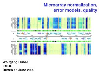
Normalization of microarray data. Anja von Heydebreck Dept. Computational Molecular Biology, MPI for Molecular Genetics, Berlin. Systematic differences between arrays. The boxplots show distributions of log-ratios from 4 red-green 8448-clone cDNA arrays hybridised with zebrafish samples.

E N D
Normalization of microarray data Anja von Heydebreck Dept. Computational Molecular Biology, MPI for Molecular Genetics, Berlin
Systematic differences between arrays The boxplots show distributions of log-ratios from 4 red-green 8448-clone cDNA arrays hybridised with zebrafish samples. Some are not centered at 0, and they are different from each other.
Systematic o similar effect on many measurements o corrections can be estimated from data Normalization Experimental variation amount of RNA in the sample efficiencies of -RNA extraction -reverse transcription -labeling -photodetection Normalization: Correction of systematic effects arising from variations in the experimental process
Ad-hoc normalization procedures • 2-color cDNA-arrays: multiply all intensities of one channel with a constant such that the median of log-ratios is 0 (equivalent: shift log-ratios). Underlying assumption: equally many up- and downregulated genes. • One-color arrays (Affy, radioactive): multiply intensities from each array k with a constant ck, such that some measure of location of the intensity distributions is the same for all arrays (e.g. the trimmed mean (Affy global scaling)).
log-log plot of intensities from the two channels of a microarray • comparison of kidney • cancer with normal • kidney tissue, • cDNA microarray with • 8704 spots • red line: median • normalization • blue lines: two-fold • change
Assumptions for normalization • When we normalize based on the observed data, we assume that the majority of genes are unchanged, or that there is symmetry between up- and downregulation. • In some cases, this may not be true. Alternative: use (spiked) controls and base normalization on them.
1. Loess normalization • M-A plot (minus vs. add): log(R) – log(G) =log(R/G) vs. log (R) + log(G)=log(RG) • With 2-color-cDNA arrays, often “banana-shaped” scatterplots on the log-scale are observed.
Loess normalization zebrafish data • Intensity-dependent • trends are modeled by • a regression curve, • M = f(A) + e. • The normalized • log-ratios are computed • as the residuals e • of the loess regression.
Loess regression • Locally weighted regression. • For each value xiof X, a linear or polynomial regression function fi for Y is fitted based on the data points close to xi. They are weighted according to their distance to xi. • Local model: Y = fi(X) + e. • Fit:Minimizethe weighted sum of squaresS wj (xj)(yj - fi(xj))2 • Then, compute the overall regression as: Y = f(X) + e, where f(xi) = fi(xi).
Loess regression regression lines for each data point The user-defined width c of the weight function determines the degree of smoothing. x0 tricubic weight function
Print-tip normalization • With spotted arrays, distributions of intensities or log-ratios may be different for spots spotted with different pins, or from different PCR plates. • Normalize the data from each (e.g. print-tip) group separately.
Print-tips correspondto localization of spots Slide: 25x75 mm 4x4 or 8x4 sectors 17...38 rows and columns per sector ca. 4600…46000 probes/array Spot-to-spot: ca. 150-350 mm sector: corresponds to one print-tip
2. Error models, variance stabilization and robust normalization
Systematic Stochastic o similar effect on many measurements o corrections can be estimated from data o too random to be ex-plicitely accounted for o “noise” Normalization Error model Sources of variation amount of RNA in the sample efficiencies of -RNA extraction -reverse transcription -labeling -photodetection PCR yield DNA quality spotting efficiency, spot size cross-/unspecific hybridization stray signal
A model for measurement error Rocke and Durbin (J. Comput. Biol. 2001): Yk: measured intensity of gene k bk: true expression level of gene k a:offset ,n:multiplicative/additive error terms, independent normal For large expression level bk, the multiplicative error is dominant. For bk near zero, the additive error is dominant.
A parametric form for the variance-mean dependence The model of Durbin and Rocke yields: Thus we obtain a quadratic dependence
Quadratic variance-vs-mean dependence data (cDNA slide) For each spot k, the variance (Rk – Gk)² is plotted against the mean (Rk + Gk)/2.
The two-component model raw scale log scale
“multiplicative” noise “additive” noise The two-component model raw scale log scale
Variance stabilizing transformations Let Xu be a family of random variables with EXu=u, VarXu=v(u). Define a transformation Var h(Xu ) independent of u
Derivation of the variance-stabilizing transformation Let Xu be a family of random variables with EXu=u, VarXu= v(u),and h a transformation applied to Xu. Then, by linear approximation of h, Thus, if h’(u)2 = v(u)-1 ,Var(h(Xu))is approx.independent of u.
1.) constant CV (‘multiplicative’) 2.) offset 3.) additive and multiplicative Variance stabilizing transformations
The “generalized log” transformation - - - f(x) = log(x) ———hs(x) = arsinh(x/s) W. Huber et al., ISMB 2002 D. Rocke & B. Durbin, ISMB 2002
A model for measurement error Now we consider data from different arrays or color channels i. We assume they are related through an affine-linear transformation on the raw scale: Yki:measured intensity of gene k in array/color channel i bki: true expression level of gene k ai, gi :additive/multiplicative effects of array/color channel i ,n: multiplicative/additive error terms, independent normal with mean 0
A statistical model • Assume an affine-linear transformation for normalization between arrays, and, after that, common parameters for the variance stabilizing transformation. The composite transformation for array/color channel i is given by ai and bi. • The model is assumed to hold for genes that are unchanged; differentially expressed genes act as outliers.
Robust parameter estimation • Assume that the majority of genes is not differentially expressed. • Userobust variant of maximum likelihood estimation: • Alternate between maximum likelihood estimation (= least squares fit) for a fixed set K of genes and selection of K as the subset of (e.g. 50%) genes with smallest residuals.
Robust normalization assumption: majority of genes unchanged • location estimators: • mean • median • least trimmed sum of squares (generalized) log-ratio
Normalized & transformed data generalized log scale log scale
Validation: standard deviation versus rank-mean plots difference red-green rank(average)
Which normalization method should one use? • How can one assess the performance of different methods? • Diagnostic plots (e.g. scatterplots) • Performance measures: • The variance between replicate measurements should be low. • Low bias: Changes in expression should be accurately measured. How to assess this (in most cases, the truth is unknown)?
Evaluation: sensitivity / specificity in quantifying differential expression o Data: paired tumor/normal tissue from 19 kidney cancers, hybridized in duplicate on 38 cDNA slides à 4000 genes. o Apply 6 different strategies for normalization and quantification of differential expression o Apply permutation test to each gene o Compare numbers of genes detected as differentially expressed, at a certain significance level, between the different normalization methods
Comparison of methods Number of significant genes vs. significance level of permutation test
Parametric vs. non-parametric normalization • Loess is non-parametric: it makes no assumptions which sort of transformation is appropriate. Disadvantage: Degree of smoothing is chosen in an arbitrary way. • vsn uses a parametric model: affine-linear normalization. Disadvantage: the model assumptions may not always hold. Advantage: If the model assumptions do hold (at least approximately), the method should perform better.
vsn may also correct “banana shape” M-A plot of vsn- normalized zebrafish data, loess fit Different additive offsets may lead to non-linear scatter plots on the log scale.
References • Software: R package modreg (loess), Bioconductor packages marrayNorm (loess normalization), vsn (variance stabilization) • W.Huber, A.v.Heydebreck, H.Sültmann, A.Poustka, M.Vingron (2002). Variance stabilization applied to microarray data calibration and to the quantification of differential expression. Bioinformatics 18(S1), 96-104. • Y.H.Yang, S.Dudoit at al. (2002). Normalization for cDNA microarray data: a robust composite method addressing single and multiple slide systematic variation. Nucleic Acids Research 30(4):e15.