Download
1 / 23
230 likes | 352 Vues
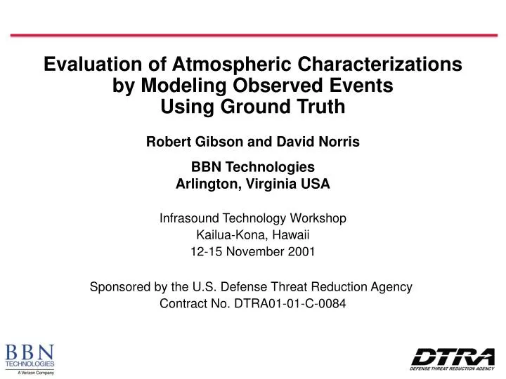
Evaluation of Atmospheric Characterizations by Modeling Observed Events Using Ground Truth. Robert Gibson and David Norris BBN Technologies Arlington, Virginia USA Infrasound Technology Workshop Kailua-Kona, Hawaii 12-15 November 2001 Sponsored by the U.S. Defense Threat Reduction Agency

E N D
Evaluation of Atmospheric Characterizations by Modeling Observed Events Using Ground Truth Robert Gibson and David Norris BBN Technologies Arlington, Virginia USA Infrasound Technology Workshop Kailua-Kona, Hawaii 12-15 November 2001 Sponsored by the U.S. Defense Threat Reduction Agency Contract No. DTRA01-01-C-0084
InfraMAP Objectives • Integrate the software tools needed to perform infrasound propagation modeling • Define the state of the atmosphere (temperature, wind) as required for input to propagation models • Predict phases (travel times, bearings, amplitudes) from atmospheric explosions as measured by infrasound sensors • Apply tools to support nuclear explosion monitoring R&D and resolve operational issues • environmental variability and propagation sensitivity • prediction of localization area of uncertainty and detection performance • performance model of an infrasound network
InfraMAP Software Schematic Azimuth Deviation Travel Time Elevation Angle Attenuation Synthetic Waveform from modes Variability Statistics Propagation Environment GUI GUI Date Time Latitude Longitude Altitude Environmental Characterization • MSIS-90 • HWM-93 • User-defined profile • Environmental Variability Propagation Modeling Near-Real-Time Updates • NRL-MSIS-00 • NRL-HWM-02 • Next Generation Model Model Parameters Source Localization Area of Uncertainty Network Performance Synthetic Phases from rays • Ray Tracing • Normal Mode • Parabolic Equation • Model-based assimilation • In-situ measurements • Solar/Magnetic parameters Network Performance Modeling GUI GUI
Development and Applications • Incorporate updated atmospheric characterizations • Determine required spatial and temporal resolutions • Evaluate best available sources • Conduct sensitivity studies • Model observed infrasound events • Obtain ground truth source location • Compare model results with observations • Assess quality of atmospheric characterization • Examples: • 23-Apr-01 Pacific Bolide • Space Shuttle launches from Kennedy Space Center
Radiosondes and Climatology • Example: Temperature profiles from seven radiosondes in SW USA
Synoptic Model and Climatology NOGAPS Meridional NOGAPS Zonal • Example: Wind profiles over 7 by 6 degree grid in SW USA
Daily Solar Flux, F10.7 (for 1998) • Solar flux and geomagnetic disturbance can affect infrasound propagation in the thermosphere • F10.7 is the daily solar radio flux at 10.7 cm wavelength, adjusted to 1 AU
Pacific Bolide: 23-Apr-01 IS10 SGAR DLIAR IS57 IS59 • Impulsive infrasound event detected at multiple stations • Nominal event location shown • Five stations used in localization analysis • Propagation through modeled atmosphere • Empirical characterizations • Spline through radiosondes
Spectrograms at Two Stations • Pacific event, 23-Apr-2001; One hour of data shown
Localization Procedure Shoot rays back from each array: Launch rays at mean observed azimuth. Fan of rays in elevation. “Reverse Propagation” Initial location estimate from ray intersections: Estimate range, travel times, signal velocities. See rays in figure below. Predict event time using each array: (Arrival time – travel time). Range of travel times determined by ray trace. Identify Eigenrays from estimated location to each array Revise location estimate Perturb location to improve consistency in event time Result of two iterations shown
Estimated Source Location From IS10 From SGAR IR / Visible (Satellites, 22 May) 27.90 N, 133.89 W From DLIAR Estimated Event Location (BBN, 18 May) 28.6 N, 134.1 W From IS57 From IS59 • Pacific event, 23-Apr-2001; Initial bundles of rays are shown • Predicted location and reported ground truth are shown
Radiosonde Locations: 23-Apr-01 Latitude (deg) Longitude (deg) Blue diamonds indicate radiosonde locations Data from circled radiosondes are shown Green Triangles are infrasound stations Source Location
Radiosondes and Climatology: 23-Apr-01 IS10 Path: Temperature DLIAR Path: Temperature IS59 Path: Temperature
Radiosondes and Climatology: 23-Apr-01 IS10 Path: Zonal IS59 Path: Zonal DLIAR Path: Zonal IS10 Path: Meridional DLIAR Path: Meridional IS59 Path: Meridional
Source Location Using In Situ Data From IS10 From SGAR IR / Visible (Satellites, 22 May) 27.90 N, 133.89 W From IS57 Estimated Event Location (BBN, w/ radiosondes) 28.7 N, 134.6 W From DLIAR From IS59 • Pacific event, 23-Apr-2001; Initial bundles of rays are shown • Ray projections shown use shooting method, not eigenrays • Localization shifted toward west
Space Shuttle - Importance of Trajectory • Infrasound from Saturn V and other rockets was observed and studied in the 60’s and 70’s • Lamont-Doherty, Palisades, NY • US Army, Ft Monmouth, NJ • Energy arrived in two bundles with different azimuths • Two source regions were identified • Rocket ascent • First stage descent • Trajectory must be understood in order to model source Typical Space Shuttle Ascent trajectory (alt. vs. time) for orbiter and solid rocket boosters
Space Shuttle Trajectories & -88 • Space shuttle trajectory depends on desired orbit • Two typical mission trajectories are shown • Example presented follows more northern trajectory • STS-96 • STS-88 • Shuttle reaches supersonic velocity approximately 1 minute after launch • Main engine cutoff occurs at 8.5 minutes after launch Trajectories determined using commercially available modeling software
Shuttle Modeling Approach • Source of infrasound is not impulsive, but continuous and moving • Approximate moving source by modeling a series of discrete events, each with appropriate time delay • Use 3-D ray tracing to find eigenrays from points on launch trajectory to infrasound array • Orbiter • Solid rocket boosters (SRB) • Determine arrival time and azimuth for each eigenray Example of eigenrays from one point on trajectory to array location
Conclusions • Software models have been successfully used to predict travel time and bearing biases for atmospheric infrasound. • Empirical atmospheric models are adequate for many scenarios, but not all. • In situ measurements demonstrate high variability of winds • Software development underway to incorporate updated atmospheric characterizations in InfraMAP. • Bolides and rocket launches are examples of model calibration sources, since ground truth may be available. • Pacific bolide example indicates complexity of modeling issues. • Space shuttle launches are a promising source of ongoing calibration data to validate environmental characterizations.