Download
1 / 33
330 likes | 465 Vues
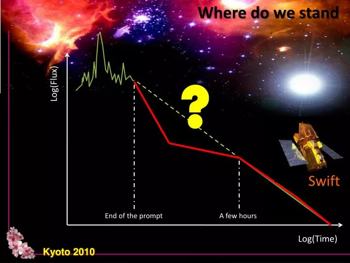
Where do we stand. ?. Log(Flux ). Swift. End of the prompt. A few hours. Log(Time ). Kyoto 2010. Log(Flux ). X-Ray Flares. Log(Time ). Kyoto 2010. GRB X- ray Flares. R. Margutti G. Chincarini , G. Bernardini , J. Mao, C. Guidorzi. Early-time flare catalog .

E N D
Where do we stand ? Log(Flux) Swift End of the prompt A few hours Log(Time) Kyoto 2010
Log(Flux) X-Ray Flares Log(Time) Kyoto 2010
GRB X-ray Flares R. Margutti G. Chincarini, G. Bernardini, J. Mao, C. Guidorzi Early-time flare catalog Late-time flare catalog Bright flare analysis t< 103s t> 103s 9 flares X-ray + gamma-ray Very good statistics 113 flares 4 different energy bands Asymmetric profile 36 flares Asymmetric profile Evolution with time (up to t≈106 s) 051117A Spectral evolution Evolution with energy band Poster: # Evolution with time Evolution with energy band Margutti et al., MNRAS accepted, Astro-ph: 1004.1568 Astro-ph: 1004.0901 As-complete-as-possible observational picture of the X-ray flare phenomenology AIM: Kyoto 2010
? GRB X-ray Flares OBSERVATIONALLY: What distinguishes a flare from a prompt pulse Do flares follow the entire set of temporal and spectral relations found from the analysis of prompt emission pulses? Width(T) Luminosity(T) Ep(t) Ep(t)-Liso(t) Ep-Liso Width(E) Lag-Lum Kyoto 2010
The Method: Trise Tdecay Width Tpeak Amplitude If with redshift: Peak Luminosity Energy Evolution with ENERGY BAND Evolution with Tpeak GRB060904B Among different flares In the same flare Kyoto 2010
Width (t) Width=trise+tdecay Width=trise + tdecay Log(width) Log(tpeak) TIME Kyoto 2010
Luminosity (t) Flares get fainter and fainter Early time sample TIME Kyoto 2010
Spectral Evolution (t) 060904B Flare: Prompt: BATSE pulse Peak Energy Time (Peng 2009) Within single flare and pulses TIME Kyoto 2010
Ep(t)-Liso(t) Ep,i (keV) Ep,i (keV) 060904B Flare 060418 Flare Liso (erg/s) Liso (erg/s) Prompt Ep,i (keV) Ghirlanda 2010 Liso (erg/s) Kyoto 2010
Ep-EisoEp-Liso Prompt data from Nava 2009 Flares Flares Kyoto 2010
Width(E) FLARES PROMPT High energy profiles peak before Flare peak Lag Kyoto 2010
Lag-Luminosity PROMPT CCF lag, time integ. 50-100 vs 100-200 keV 1-10000 keVLpeak (Ukwatta 2010) Norris 2000 relation Peak lag, flares 0.3-1vs 3-10 keV 0.3-10 keVLpeak (Margutti 2010) FLARES Kyoto 2010
Summary: Flares paradigm High energy flareprofiles rise faster, decay faster and peak before the low energy emission. FLARES EVOLVE WITH TIME As time proceeds flares become wider, with larger peak lag, lower luminosities and softer emission. Kyoto 2010
Summary: FLARES EVOLVE WITHTIME Margutti 2010 FLARES PROMPT Width(T) Luminosity(T) Ep(t) Ep(t)-Liso(t) Ep-Liso Width(E) Lag-Lum ≈const ≈const ≈similar ? Kyoto 2010 Astro-ph: 1004.1568 Astro-ph: 1004.0901
THANK YOU!! Kyoto 2010
BAT-XRT spectral index BAT XRT