Download
1 / 35
360 likes | 514 Vues
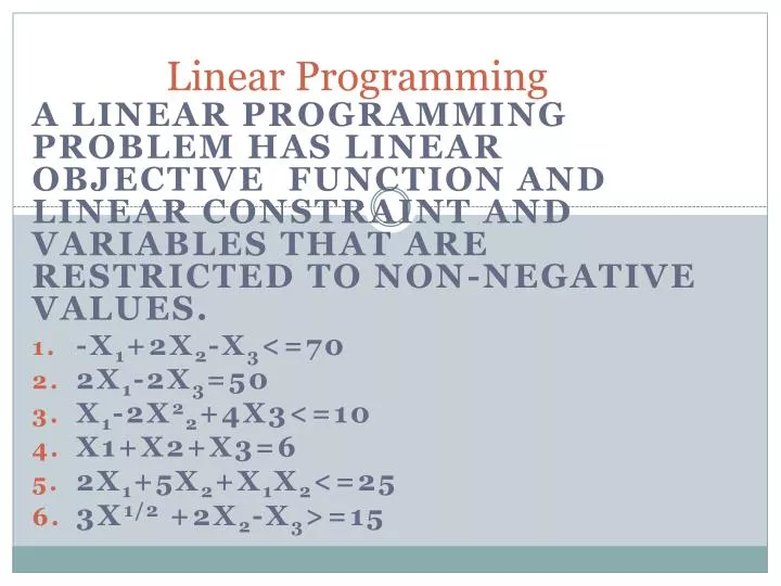
Linear Programming. A linear programming problem has linear objective function and linear constraint and variables that are restricted to non-negative values. -X 1 +2X 2 -X 3 <=70 2X 1 -2X 3 =50 X 1 -2X 2 2 +4X3<=10 X1+X2+X3=6 2X 1 +5X 2 +X 1 X 2 <=25 3X 1/2 +2X 2 -X 3 >=15.

E N D
Linear Programming A linear programming problem has linear objective function and linear constraint and variables that are restricted to non-negative values. -X1+2X2-X3<=70 2X1-2X3=50 X1-2X22+4X3<=10 X1+X2+X3=6 2X1+5X2+X1X2<=25 3X1/2 +2X2-X3>=15
Linear Programming Feasible solution: The solution of the problem that satisfy every constraint is called as feasible solution. For constraint <=0 feasible solution lie under the constraint For constraint >=0 feasible solution above under the constraint For constraint ==0 feasible solution lie on constraint .
Graphical Method Prepare a graph for the feasible solutions for each of constrains. .Determine the feasible region by identifying the solutions that satisfy all constrain simultaneously. . Draw an objective function line showing the values of the decision variable yield a specified value of objective function. A Linear programming problem involving two variables can be solved using the graphical solution
Graphical Method Move parallel objective function lines toward larger objective function values until further movement would take the line completely out of feasible region Any feasible solution on objective function line with the largest value is an optimal solution
Summary of the Graphical Solution Procedurefor Maximization Problems Prepare a graph of the feasible solutions for each of the constraints. Determine the feasible region that satisfies all the constraints simultaneously.. Draw an objective function line. Move parallel objective function lines toward larger objective function values without entirely leaving the feasible region. Any feasible solution on the objective function line with the largest value is an optimal solution.
Problem A small manufacturing company decided to move in market for standard and deluxe golf bags. Initial analyses showed that each bag produced will require following operation 1.cutting and dyeing material 2.sweing 3.Finishing 4.Inspection and packing
Problem For a standard bag each bag will require: 7/10 hr in cutting & dyeing, 1/2 hr in sewing 1 hr in finishing department 1/10 hr in inspection For a high -priced bag each bag will require : 1 hr in cutting & dyeing, 5/6 hr in sewing 2/3 hr in finishing department 1/4 hr in inspection
Decision Making Price for profit contribution standard bags $10, Price for Deluxe bag is $9.
Problem How many constraints are in this problem. How many decision variable are in this problem what is objective function.
Problem formulation Max 10S +9D s.t 7/10S+1D<=630 (Cutting & dyeing) 1/2S+5/6D <=600 Sewing 1S+2/3D<=708 Finishing 1/10S+1/4D<=135 Inspection & Packaging
Solutions . Prepare a graph for the feasible solutions for each of constrains. How? Take S on x-axis and D on Y-axis For each constrain put S= 0 Get D to obtain a point (0,D) then put D=0 Get S to obtain (S,0) , join these two point to get the line.
Cutting and Dyeing Constrain Constrain Equation: 7/10S+1D<=630 Solve for equality first by determining two points as described above: 7/10S+1D=630 S=0 -> D=630, D=0 -> S=900 Points (0,630) and (900,0)
Cutting and Dyeing Constrain Find the points lie above the feasible region
Other Constraints 1/2S+5/6D <=600 (Sewing) Points ???? 1S+2/3D<=708 (Finishing) Points???? 1/10S+1/4D<=135 (Inspection & Packaging) Points?????
Feasible Solutions as Profit increases Let us take any arbitrary profit and draw it on feasible solution 10S+ 9D=1800; (putting S, D 0) find points 10S+ 9D=3600 10S+9D=5400
Feasible Solutions V/S Profit Profit lines are parallel to each other, higher value of the objective for higher profit lines, However at some value line would be outside the feasible region. The point in the feasible region that lies on highest profit line is optimal solution.
Feasible Solutions V/S Profit Intersection of cutting & Dyeing and finishing constraint gives an optimal solution. 7/10S+1D<=630 (Cutting & dyeing) 1S+2/3D<=708 Finishing Find point of intersection and check the profit for the optimal solution. 10s+9d=???
Slack Variables Any unused capacity for a<=constraint is called as slack variables Putting the value of the optimal solution in all constraint
Slack and Surplus Variables A linear program in which all the variables are non-negative and all the constraints are equalities is said to be in standard form. Standard form is attained by adding slack variables to "less than or equal to" constraints, and by subtracting surplus variables from "greater than or equal to" constraints. Slack and surplus variables represent the difference between the left and right sides of the constraints. Slack and surplus variables have objective function coefficients equal to 0.
Standard Form Add four slack variables to constraint having zero coefficient for unused capacity. Max 10S+9D+0S1+0S2+0S3+0S4 7/4S + 1D + 1S1=630 1/2S+5/6D +1S2=600 1S+2/3D +1S3=708 1/10S+1/4D +1S4=135 S1=0,S2=120,S3=0,S4=18
Extreme Points The vertices of feasible region is called as vertices of the feasible region. It has 5 extreme points. Optimal solutions occur at one of vertices of the feasible solutions, one producing highest value of objective function is the required optimal solution.
II. Objective function: Max 5S+ 9D What about constraints Check the objective function at the extreme points. S=300,D=420 find objective function S=540,D=252 find objective function Which one produce max objective function..
Alternative Optimal Solution III. Max 6.3S +9D Check the objective function at the extreme points. S=300,D=420 find objective function S=540,D=252 find objective function
Infeasibility Suppose if management want to produce at least S=500 and D=360 with the same given constraints Then there would be no feasible region
Minimization Problem A company sales two products A and B. The combined production for production A and B must be at least 350 gallons. Additionally a major customer require 125 gallon of Product A. Product A requires 2 hrs and product B requires 1 hr of processing time per gallon respectively. Total 600 processing hrs is available Production cost is $2 gallon and $3 gallon for A and B respectively. Objective function & constraint
Minimization Problem Min 2A+3B 1A>=125 (demand for A) 1A+1B>=350 (Total Production) 2A+1B<=600 (Processing Time) A,B>=0
Feasible Region Find Extreme point using intersection of three lines 1.(A,B)=(125,225) 2.(A,B)=(125,350) 3.(A,B)=(250,100)
Optimal solution: Objective function: 2A+3B 2(125)+3(350)=1300 2(125)+3(225)=925 2(250)+3(100)=800
Example: Unbounded Problem Solve graphically for the optimal solution: Max 3x1 + 4x2 s.t. x1 + x2> 5 3x1 + x2> 8 x1, x2> 0
Example: Unbounded Problem The feasible region is unbounded and the objective function line can be moved parallel to itself without bound so that z can be increased infinitely. x2 3x1 + x2> 8 8 Max 3x1 + 4x2 5 x1 + x2> 5 x1 2.67 5