Download

1 / 66
670 likes | 845 Vues
Chesapeake Bay Program Modeling Past, Present, and Future. Chesapeake Bay Program Office. The Chesapeake Bay and Watershed. Forest 64% Agricultural 24% Urban 8% Other 4%. Ratio of Areas Watershed : Estuary ~ 15:1. Effects of Excess Sediment. Can damage habitats of some

E N D
Chesapeake Bay Program ModelingPast, Present, and Future Chesapeake Bay Program Office
The Chesapeake Bay and Watershed Forest 64% Agricultural 24% Urban 8% Other 4% Ratio of Areas Watershed : Estuary ~ 15:1
Effects of Excess Sediment Can damage habitats of some Plants and animals. Excess sediment can cloud water, block sunlight, and cause SAV to die.
Effects of Excess Nutrients When excess algae die and decompose, they use up oxygen in the water that plants and animals need to survive. Excess algae cloud water, block sunlight, and cause SAV to die.
The Chesapeake Bay Program Partnership Governor of MD Governor of PA Governor of VA Mayor of DC EPA Administrator Executive Council Chair of Chesapeake Bay Commission
Reduce Nutrient Pollution Loads As we reduce loads... …we increase achievement of water quality conditions.
Chesapeake Bay Program Management Questions • What is the estuarine response to reductions of nutrients and sediment? • Water quality (dissolved oxygen) • Living resources (crabs and fish) • What reductions are achievable? • What to do • Where to do it • Changes in loads from management actions • What are the local effects on riverine water quality?
Chesapeake Bay ProgramDecision Support System Land Use Change Model Criteria Assessment Procedures Bay Model Watershed Model Management Actions Scenario Builder Airshed Model Sparrow Effects Allocations
Chesapeake Bay ProgramDecision Support System Land Use Change Model Criteria Assessment Procedures Bay Model Watershed Model Management Actions Scenario Builder Airshed Model Sparrow Effects Allocations
Hourly Values: Rainfall Snowfall Temperature Evapotranspiration Wind Solar Radiation Dewpoint Cloud Cover Snapshot: Land Use Acreage BMPs Fertilizer Manure Atmospheric Deposition Point Sources Septic Loads Quick Overview of Watershed Model Scenarios Hourly output is summed over 10 years of hydrology to compare against other management scenarios 1991-2000 HSPF “Average Annual Flow-Adjusted Loads” 12
Each segment consists of separately-modeled land uses High Density Pervious Urban High Density Impervious Urban Low Density Pervious Urban Low Density Impervious Urban Construction Extractive Wooded Disturbed Forest Corn/Soy/Wheat rotation (high till) Corn/Soy/Wheat rotation (low till) Other Crops Alfalfa Nursery Pasture Degraded Riparian Pasture Animal Feeding Operations Fertilized Hay Unfertilized Hay Nutrient management versions of the above Plus Point Source and Septic 13
Different Types of Load Allocations to Sources Source Land Use of origin 14
From the Chesapeake Bay Commission Report: Cost-Effective Strategies for the Bay December, 2004
First Version of the Watershed Model: • Completed in 1982. • 63 model segments. • 2 year calibration period • (Mar.- Oct.). • 5 land uses. • IBM mainframe platform.
Primary Products of the First Version of the Watershed Model: First estimate of relative point source and NPS loads for each major basin. Demonstration of the importance of controlling NPS loads in the Chesapeake. "Framework for Action" report, the first basin by basin assessment of Chesapeake nutrient loads.
Second Version of the Watershed Model - Phase 2: • Completed in 1992. • 63 model segments. • 4 year calibration period (1984-87). • 9 land uses. • DEC VAX mainframe platform.
Primary Products of Phase 2: • First nitrogen and phosphorous allocations for each major basin. • First linkage to water quality model of the estuary. • First linkage to the airshed model (RADM) and estimates of atmospheric loads for each major basin.
Third Version of the Watershed Model - Phase 4: • Completed in 1998. • 94 model segments. • 9 land uses. • 14 year calibration period (1984-97) using automated input and output model processors. • Cray, DOS, Solaris, and linux platforms.
Primary Products of Phase 4: • Nutrient Allocations in 2000 (p4.1) • Nutrient Allocations in 2003 (p4.3) • Began open source, public domain, web distribution of preprocessors, post processors, and open source code. First download and use by non-CBP.
Fourth Version of the Watershed Model - Phase 5: • 1,063 model segments. • 21 year calibration period (1985-2005). • 24 land uses using • time-varying land use & BMPs. • Open source, public domain, distributed over the web: • http://ches.communitymodeling.org/models/CBPhase5/index.php • Purpose: TMDL
Automated Calibration Calibration Procedures Input Data “Scenario builder” Calibration Data 24
Phase 5 – A Ten Fold Increase in Segmentation Over Previous Phase 4.3 Model Phase 4.3 land and river segments Phase 5 land segments Phase 5 river segments
A software solution was devised that directs the appropriate water, nutrients, and sediment from each land use type within each land segment to each river segment External Transfer Module Each land use type simulation is completely independent. Each river simulation is dependent on the local land use type simulations and the upstream river simulations.
Flexible Functionality WDM = HSPF-specific binary file type UCI = User Controlled Input (input file) MET WDM ATDEP WDM PS WDM Land Input File Generator River Input File Generator 4 1 External Transfer Module 2 3 5 Land variable WDM River variable WDM Final Text Output 6 • Land UCIs are generated • HPSF is run on the land UCIs and output is stored in individual WDMs • The ETM is run converting land output to river input, incorporating land use, BMPs, and land-to-water delivery factors. Output is stored in river-formatted WDMs • River UCIs are generated • HSPF is run on the river UCIs and output is written back to WDMs • Postprocessor reads river WDMs and writes ASCII output
Chesapeake Bay ProgramDecision Support System Land Use Change Model Criteria Assessment Procedures Bay Model Watershed Model Management Actions Scenario Builder Airshed Model Sparrow Effects Allocations
Number of Scenarios • Phase 1 – 0 • Phase 2 – fewer than 10 • Phase 3 – never used • Phase 4.1 – 37 • Phase 4.3 – 400-500 • Phase 5 – about 30 pre-finalization • Lauren Hay plans to run 600 • 1000s? For management
Watershed Wide Crops by Acreage Tracking yields and acreages on a county basis Approximately 100 crop types and 10 growing regions with different parameters for each 32
Manure Data Model Runoff Transport Volatilization Volatilization Volatilization Uncollected Pasture Volatilization Beef Dairy Collected Swine Enclosure Daily Application Layers Broilers Turkeys Storage Crop Spring/Fall Application Volatilization Barnyard Daily Application Runoff
Volatilized fertilizer NH3 Fertilizer Sold NM crops w/o manure NM acres w/ manure starter fertilizer, with manure applied after Manure on NM acres Acres of crop w/o manure Non-NM acres Manure Mass-balance Non-NM acres w/ all leftover fertilizer Non-NM acres w/ leftover manure 34
Chesapeake Online Assessment Support Tool Choose your task Select Your Watershed Scenario Builder View loads spatially Observed Data and Calculated Trends View Factors Affecting Trends Product of USGS and CBPO
Chesapeake Bay ProgramDecision Support System Land Use Change Model Criteria Assessment Procedures Bay Model Watershed Model Management Actions Scenario Builder Airshed Model Sparrow Effects Allocations
Inorganic Carbon Respiration Respiration Three Algal Groups Microzooplankton Mesozooplankton Respiration Dissolved Organic Carbon Labile Particulate Organic Carbon External Loads Refractory Particulate Organic Carbon Sediments Carl Cerco USACE - ERDC
The 1987 Model • 3-D hydrodynamics and water quality. • Summer, steady-state. • Indicated the importance of sediment-water interactions. • One part of decision process that concluded a 40% nutrient load reduction would eliminate anoxia. 1985 grid, 585 cells
Three-D Time Varying Model (1992) • Linked watershed, hydrodynamic, and eutrophication models. • Dynamic benthic sediment diagenesis component. • Continuous application 1984-1986 and 1959-1988. • Guided 1991 re-evaluation of 1987 Chesapeake Bay Agreement. 1992 grid, 5000 cells
Tributary Refinements 1997 • 10,000 cell grid. • Intertidal hydrodynamics. • Ten-year simulation 1985-1994. • Direct simulation of living resources.
Tributary Refinements 1997 • Move boundary out to continental shelf. • Introduce suspended solids. • Relate light attenuation to suspended solids.
Added Living Resources 2003 • 13,000 cells • Mesozooplankton • Microzooplankton • Submerged Aquatic Vegetation • Filter Feeding Benthos (three species) • Deposit-Feeding Benthos
Inorganic Carbon Respiration Respiration Three Algal Groups Microzooplankton Mesozooplankton Respiration Dissolved Organic Carbon Labile Particulate Organic Carbon External Loads Carbon Cycle Refractory Particulate Organic Carbon Sediments
Epiphytes Phytoplankton SAV Shoots Dissolved Nutrients Particulate Nutrients Water Column Sediments SAV Roots Dissolved Nutrients Particulate Nutrients Submerged Aquatic Vegetation Model
Particulate Organic Matter respiration filtration Dissolved Nutrients Dissolved Oxygen excretion settling Water Column Filter Feeders Sediments sediment-water exchange sediment-oxygen demand biodeposits Particulate Organic Matter Dissolved Nutrients diagenesis excretion Oxygen Demand diagenesis feeding Deposit Feeders respiration Benthic submodel
The 2008 Model • 57,000 total cells. • Process-oriented suspended solids model with ROMS bed. • Advanced optical model. • oyster model. • Menhaden model