Download
1 / 42
420 likes | 481 Vues
Memory Management (Ch. 8). Compilers generate instructions that make memory references. Code and data must be stored in the memory locations that the instructions reference. How does the compiler know where the code and data will be stored?

E N D
Compilers generate instructions that make memory references. • Code and data must be stored in the memory locations that the instructions reference. • How does the compiler know where the code and data will be stored? • When code and data are stored, what if the memory locations the instructions reference are not available?
Background • Absolute code: • Compiler knows where code will reside in memory. • Creates memory references in instructions based on where code will reside. • Also called Compile time binding. • Give assembly-type example showing some load/add instructions.
Relocatable code: • binding of code to real memory locations done at load time. • Also called load time binding.
Execution time binding: • binding of code to real memory during execution. Allows load modules to be moved.
Physical address: • Actual memory location in the memory chip that is referenced. • Logical address (sometime called virtual address): • Memory location specified in an instruction. • May not be the same.
Base register approach. • See figures 8.1-8.4: • physical address = logical address + contents of base register. • Used in IBM 360/370 architectures – a milestone in computer architecture.
Set of addresses defines the logical address space or the physical address space. • Assumes entire process loaded into memoryconstraints on process size. • Dynamic loading: code sections loaded into memory as needed. • Static linking: object code and libraries combined into one executable to create a large file.
Dynamic linking: Executable contains a stub (small piece of code that locates the real library) for each library routine. • Overlays: Sections of code that occupy the same memory but never at the same time. • Discuss using hierarchical structures. • Used in older systems
Swapping: • All or parts of processes are moved between memory and disk. • Moved into memory when needed • Moved to disk when not needed • Backing store: • Temporary area (usually disk) for a running process’ code. • Fig. 8.5
CPU Scheduler calls a dispatcher which checks to see if process code is in memory. • If not, swap in and replace another process if necessary. • See example equation for context switch time on page 315.
Contiguous memory allocation • Memory protection: • Logical address < contents of a limit register; • physical address=logical address + relocation register. • Figure 8.6.
Fixed partitions: • Memory divided into fixed length partitions. • Process code stored into a partition. • Internal fragmentation (unused part of a partition). • Finding the best partition: first fit, best fit,
Variable partitions: • OS creates partitions as processes are loaded. • External fragmentation: many small unused partitions • compacting: moving all free partitions to adjacent areas of memory. • Coalescing: combing adjacent partitions. • More overhead as OS creates, compacts, and coalesces partitions.
Paging • Prior schemes try to configure memory to fit a process. • Why not try to configure a process to fit memory? • Code divided into pages. • Memory divided into frames.
Logical address: (p, offset). • P is the page number; offset is the relative byte position on that page • Page table: table that associates a frame with each page • p (page number) indexes a page table to get a frame number, f. • Physical address is (f, offset).
Figure 8.7-8.10. • Need a page table base register to locate the page table. • Offset is n bits if the page size is 2n.
Pages need not be stored in contiguous memory. • NO external fragmentation; internal fragmentation possible. • OS maintains a free-frame list/frame table. • Size of memory= number of frames * size of frame (anywhere from ½ K to about 8K.
Translation look-aside buffer (TLB) • Page table access would mean double memory references. • TLBs: hardware registers that associate a page # with a frame #. • Instruction cycle checks TLB first; if page not found, then access the page table. • Figure 8.11
Spatial locality: • If a memory location is referenced then it is likely that nearby locations will be referenced. • Temporal locality: • If a memory location is referenced then it is likely it will be referenced again. • Means that TLB searches will be successful most of the time.
Hit ratio (H): • Frequency with which page# found in TLB. • Effective memory-access time: • H*(time to access TLB and memory) + (1-H)*(time to access page table and memory). • See book for numbers (p. 326)
NOTE: OS may run in unmapped mode, making it quicker. • TLB reach: metric defined by amount of memory accessible through the TLB • (# entries*page_size).
Protection bits • Bits associated with each frame • stored in page table. • Control type of access (read, write, execute, none). • Discuss (not in book).
Valid/Invalid bit. • Bit in page table indicating whether page referenced is valid (in memory). • Figure 8.12 • tradeoffs: • small page size: less fragmentation but more pages and large page tables. • large page size: the reverse.
Shared memory • Two (or more) process’ virtual memory can map to the same real memory. • Common examples of sharing code (compilers, editors, utilities). • Example: if everyone is using vi, could use a lot of memory if vi not shared. • Figure 8.13. • Program demos show how to do this. (later).
Linux Shared memory demos • Shared memory commands: see ftok(), shmget(), shmat(), shmdt(), and shmctl()in the Linux list of command provided via the course web site. • Compile getout1.c and call it getout. • Compile putin1.c and run.
The putin program creates a shared memory segment and writes to it. It also forks and execs the getout program. • The getout program displays the constents of the shared memory segment.
Remove the comments in putin’s loop that writes to the shared memory segment. • Run the program several times. • Comment out the shmctlcommand at the end of the putout program. • What happens?
Bash shell command: ipcs – reports on interprocess communication facilities. • Bash shell command: ipcrm – can remove one of the IPC facilities that may be “orphaned”. • The shell script removeshm makes this easier to do.
Programs putin2.c and getout2.c are an attempt at synchronizing multiple instances of writing to and reading from shared memory. • Sometimes it works!!
Storing (structuring) the page table • Page table could have a million entries. Can’t store contiguously. • Two level paging
p1: identifies an outer page table entry, which locates an inner page table • p2: identifies an inner page table entry, which locates the frame number • Used in some Pentium machines; 12-bit offset 2K-byte page size. 10 bits for each of p1 and p2.
Sometimes called forward-mapped page table. • Figs 8.14-15.
VAX architecture • 512-byte page sizes. Outer page actually called a section.
other examples: • Use a 3-level hierarchy (SPARC) architecture or even 4-level (Motorola 68030).
Hashed page table • Virtual page number acts as a hash value, not an index. • Hash value identifies a list of (p#, f#) pairs. • Fig. 8.16.
Inverted page table • Previous approaches assume one page table for each process and one entry for each virtual page. Over many processes, this could require many entries. • inverted page table: • one entry for each frame. • Each entry contains a virtual page # and process ID of the process that has that page. • Fig 8.17
Used by PowerPC and 64-bit UltraSPARC. • Virtual address looks like • Look for virtual address in TLB. • If not found, search (actually use a hash on (pid, p#) ) inverted page table looking for (pid, p#). • If found, extract f#.
Segmentation • Paging requires a view that is simply a sequence of pages. • Segmentation allows a more flexible view: data segment, stack segment, code segment, heap segment, standard C library segment • Segments vary in size.
Pure segmentation works much like paging (use segment table, not page table and segment #, not page #) except segment sizes vary. Segment table entry contains segment address and its size. • Diagrams are similar. See book. Figs 8.19-8.20
Segmentation/paging • Can protect many pages the same way using protection bits on a segment table entry. Facilitates security – one entry protects an entire segment • Common on Intel chips. • Book describes 80x86 address translation but I won’t cover.
reference[http://en.wikipedia.org/wiki/Virtual_memory#Windows_example]reference[http://en.wikipedia.org/wiki/Virtual_memory#Windows_example] • Pentium and Linux on Pentium Systems (Sections 8.7.2-8.7.3)