Download
1 / 9
90 likes | 193 Vues
LHC-HCG meeting. Matters of convention for “expected” results. 1. Mean vs. median vs. Asimov 2. How do we define 1 s and 2 s bands ?. Mingshui Chen. A few examples. Differential distributions of CL.95% upper limits (Bayesian with flat prior) for 1000 sets of outcomes.

E N D
LHC-HCG meeting Matters of convention for “expected” results 1. Mean vs. median vs. Asimov 2. How do we define 1s and 2s bands ? Mingshui Chen Jan 27, 2011 Mingshui Chen ( University of Florida ) 1
A few examples Differential distributions of CL.95% upper limits (Bayesian with flat prior) for 1000 sets of outcomes 3. Multiple channels with small statistics two channel, no systematics nsig1=0.3 nbkg1=3 nsig2=0.5 nbkg2=1 The discrete probabilities will NOT be changing smoothly as one moves along r from small to large r, due to the dips 2. Single channel with small statistics nbkg=1, nsig=1, no systematics The discrete probabilities will be changing smoothly as one moves along r from small to large r 1. Large statistics nbkg=100, nsig=50, no systematics Discreteness of lines hardly seen Jan 27, 2011 Mingshui Chen ( University of Florida ) 2
Mean or Median or “Asimov” • Do we show "mean" • well defined, requires almost no conventions • but statisticians do not like "mean" as it is not “preserved” under transformations of variables; but do we really care? • or "median" • requires a convention for highly discrete distributions • or “Asimov data" ? • “imaginary” (in general, non-integer) most probable experimental outcome • requires a whole paragraph of explanations Jan 27, 2011 Mingshui Chen ( University of Florida ) 3
Conventions of bands • A simple naïve convention • ±1 and ±2 standard deviation (“two sided”) spread of the expectation obtained from a large number of toy experiments • It becomes rather problematic for small statistics cases where bands must be asymmetric and even one-sided… • Build up CL intervals by adding up probability-ranked possible experimental outcomes • If p(r) changes smoothly, say first rising up and then falling down, then one would get a continuous interval. • If probabilities are jumping up and down, such procedure would give disjoint sections as in the case of multiple channels with small statistics • Build up CL intervals following “quantiles” using cumulative distributions • see next slides • Build up CL intervals following minimum-range principle • see next slides • We need a well-defined convention Jan 27, 2011 Mingshui Chen ( University of Florida ) 4
Convention of bands in LandS • Throw 1000 toy experiments according to the background-only model (use bkgd systematic errors when non-zero) • Evaluate r95% for each of the 1000 toy experiments • Make differential and cumulative distributions of the obtained r95% values differential distribution of r95% cumulative distribution of r95% 0.977 0.841 0.5 (median) 0.159 0.023 To define median/bands, use crossings of the percentile lines and the interpolation line between nearby pairs of physically possible values of r. The current interpolation choice is the Fermi function average expected <r> Jan 27, 2011 Mingshui Chen ( University of Florida ) 5
Bands with different interpolations nbkg=1, nsig=1, no systematics, Bayesian with flat prior Fermi function interpolation Step function Linear interpolation - 2s = 3.00 - 1s = 3.00 median = 3.45 +1s = 4.73 +2s = 6.67 - 2s = 3.00 - 1s = 3.00 median = 4.11 +1s = 5.41 +2s = 6.78 - 2s = 3.00 - 1s = 3.00 median = 3.46 +1s = 4.88 +2s = 6.72 Jan 27, 2011 Mingshui Chen ( University of Florida ) 6
Bands with minimum-range principle • E.L. Crow and R.S. Gardner,Confidence intervals for the expectation of a Poisson variable, Biometrika 46 (1959), pp. 441–453. • From the differential distribution of r95% , get all intervals which contain 68%/95% ofpossible limits • e.g. on right plot, both ranges • [4.1, 7.7]and [4.6, 9.4] • contain 68% of possible limits • Take the interval corresponding to minimum range Jan 27, 2011 Mingshui Chen ( University of Florida ) 7
An example with different conventions • s = b = 10 / (m/100)^2 • no systematics, Bayesian with flat prior • With interpolation "mean“ (blue solid) and "Asimov" (red solid) are the same for all three plots • Minimum-range principle • Step function Jan 27, 2011 Mingshui Chen ( University of Florida ) 8
Summary: possible options to choose from "Typical" expected result : "Green"/"yellow" bands require convention, e.g. Jan 27, 2011 Mingshui Chen ( University of Florida ) 9