Download
1 / 20
200 likes | 340 Vues
Hydrologic modeling of Waller Creek. Prepared by: Mustafa AKCAY. TABLE OF CONTENTS. BACKGROUND WORKING WITH HEC-Prepro RUNNING HMS CALIBRATION OF HMS PARAMETERS RESULTS CONCLUTION. BACKGROUND HYDROLOGIC SYSTEM MODEL.

E N D
Hydrologic modeling of Waller Creek Prepared by: Mustafa AKCAY
TABLE OF CONTENTS BACKGROUND WORKING WITH HEC-Prepro RUNNING HMS CALIBRATION OF HMS PARAMETERS RESULTS CONCLUTION
BACKGROUND HYDROLOGIC SYSTEM MODEL HSM is an approximation of the actual system in which inputs and outputs are measurable hydrologic variables and system operator is described by a set of equations linking the inputs and outputs. Input Output I(t) Q(t) Q(t)= I(t) Operator,
Hydrologic Model Classification System f(ran.,space,time) Hydrologic Models Physical Models Abstract Models Input Output HMS (Hydrologic Modeling System) Deterministic Stochastic Output is not a fixed Input F(infiltration,transform,routing) Output value but instead described as a Precipitation, i Stream flow,Q probability distr.
RUNNING HEC-Prepro • Dem Digital Elevation • RF3 Stream Network
BURNING IN FILLING STREAM GRIDSFLOW DIRECTION FLOW ACCUMULATION • Rising the land surface cells that are of stream to delinate streams from DEM. • Filling the pits that are probably to cause wrong flow directions • Defing threshold or minimum drainage area • Darker the color of individual grid,the more grid cells drain into that cell.
GAGES--OUTLETS--LINKSSUB-WATER DELINEATION VECTORIZATION • Shape file with points representing gages that will be imported into ArcView. • Adding outlets to change the places of gages that are off the river and pointing the joints • Delineation of watershed according to gages,outlets,links • Vectorization for easyness of using and storing data compared with grid base analysis.
RUNNING HMSRUNNING HMS Transfer of Hydrologic Attributes to Schematic Creating the HMS Components • HMSschematic is conceptual model that captures the connectivity between the different elements of the hydrologic system • Opening a new HMS project and importing the basin file , and then adding a background map .
Location of USGS Stations ,38th street and 23rd street, and their annual peak values for corresponding rainfall.
Application of Rational Method • Assumptions: • Computed peak rate of runoff at the outlet point is a function of the average rainfall rate during the time of concentration. • Time of concentration: Time from most remote part of the drainage area to the out flow point. • Constant rainfall intensity.
Most critical flow between 1959-64Q1(HMS)=173cfs Q1(Measured)=289cfs 40%accuracyQ2(HMS)=295cfs Q2(Measured)=717cfs 143% accuracy
Most Critical Flow Between 1965-1972 Q1(HMS)=366.9cfs Q1(Measured)=589 60% accuracy Q2(HMS)=633cfs Q2(Measured)=857 35% accuracy
Most Critical Flow Between 1973-1979 Q1(HMS)=614cfs Q1(Measured)=521cfs 15% accuracy Q2(HMS)=1059cfs Q2(Measured)=1386cfs 30% accuracy
RESULTS • According to data I obtained, by the definition of stochastic model; • the runoff will fall in 140%, 60%, 30% neighborhood of runoff you obtained from HMS between 1959-64, 1965-72, 1973-1979 respectively. • For runoff from 1997-... ?
CONCLUSION • Using SCS Method for Infiltration may increase the precision of the model. • Lots of uncertainty affecting the output so it is difficult to make modeling with high accuracy • Don’t even think of a modeling of a basin by just one rainfall gage station!
Appreciations • Esteban AZAGRA • Jona F.JONSDOTTIR