Download
1 / 90
940 likes | 1.19k Vues
According to the theory of electricity and magnetism, a spinning charge generates a magnetic field, and it is this motion that causes the electron to behave like a bar magnet. Evidence for electron spin comes from the Stern- Gerlach experiment. Summary. Summary.

E N D
According to the theory of electricity and magnetism, a spinning charge generates a magnetic field, and it is this motion that causes the electron to behave like a bar magnet. Evidence for electron spin comes from the Stern-Gerlach experiment.
Summary quantum numberinfo obtained
Summary quantum numberinfo obtained n size, energy
Summary quantum numberinfo obtained n size, energy l shape
Summary quantum numberinfo obtained n size, energy l shape ml orientation
Summary quantum numberinfo obtained n size, energy l shape ml orientation msconveys information on possible pairing of electrons in orbitals.
Atomic Orbitals An orbital is related to the probability function, which in turn depends on the wave function .
Atomic Orbitals An orbital is related to the probability function, which in turn depends on the wave function . Each wave function describes an electron (or electrons) characterized by the quantum numbers n, l, ml, and ms.
Names of orbitals Quantum numbers Orbital name
Names of orbitals Quantum numbers Orbital name n = 1, l = 0 1s
Names of orbitals Quantum numbers Orbital name n = 1, l = 0 1s n = 2, l = 1 2p
Names of orbitals Quantum numbers Orbital name n = 1, l = 0 1s n = 2, l = 1 2p n = 3, l = 2 3d
Names of orbitals Quantum numbers Orbital name n = 1, l = 0 1s n = 2, l = 1 2p n = 3, l = 2 3d n = 4, l = 3 4f etc.
Relation Between Quantum Numbers and Atomic Orbitals nShelllmlTotal number atomic value valuevalueof orbitalsorbitals
Relation Between Quantum Numbers and Atomic Orbitals nShelllmlTotal number atomic value valuevalueof orbitalsorbitals 1 K 0 0 1 1s
Relation Between Quantum Numbers and Atomic Orbitals nShelllmlTotal number atomic value valuevalueof orbitalsorbitals 1 K 0 0 1 1s 2 L 0 0 1 2s
Relation Between Quantum Numbers and Atomic Orbitals nShelllmlTotal number atomic value valuevalueof orbitalsorbitals 1 K 0 0 1 1s 2 L 0 0 1 2s 1 -1, 0, 1 3 2px, 2py, 2pz
Relation Between Quantum Numbers and Atomic Orbitals nShelllmlTotal number atomic value valuevalueof orbitalsorbitals 1 K 0 0 1 1s 2 L 0 0 1 2s 1 -1, 0, 1 3 2px, 2py, 2pz 3 M 0 0 1 3s
Relation Between Quantum Numbers and Atomic Orbitals nShelllmlTotal number atomic value valuevalueof orbitalsorbitals 1 K 0 0 1 1s 2 L 0 0 1 2s 1 -1, 0, 1 3 2px, 2py, 2pz 3 M 0 0 1 3s 1 -1, 0, 1 3 3px, 3py, 3pz
Relation Between Quantum Numbers and Atomic Orbitals nShelllmlTotal number atomic value valuevalueof orbitalsorbitals 1 K 0 0 1 1s 2 L 0 0 1 2s 1 -1, 0, 1 3 2px, 2py, 2pz 3 M 0 0 1 3s 1 -1, 0, 1 3 3px, 3py, 3pz 2 -2, -1, 0, 1, 2 5 3dxy, 3dyz, 3dxz ,
s orbitals It is convenient to think of the charge cloud corresponding to each particular orbital as having a certain shape – though strictly speaking, the charge cloud corresponding to each orbital does not have a well defined shape.
s orbitals It is convenient to think of the charge cloud corresponding to each particular orbital as having a certain shape – though strictly speaking, the charge cloud corresponding to each orbital does not have a well defined shape. This is due to the fact that the orbital actually extends from the nucleus to infinity.
Roughly speaking, there is about a 90% probability of finding the electron within a sphere of radius 1 Å surrounding the nucleus (Å = Angstrom, 1 Å = 1 x 10⁻¹⁰m)
Roughly speaking, there is about a 90% probability of finding the electron within a sphere of radius 1 Å surrounding the nucleus (Å = Angstrom, 1 Å = 1 x 10⁻¹⁰m) It is useful to represent the 1s orbital by drawing a boundary surface diagramthat encloses about 90% of the total electron density.
Radial probability distribution Radial probability distribution: In simplified terms, this determines the probability that a particle (i.e. an electron) will be found in a spherical shell of thin thickness at a distance r from the nucleus.
A 2s orbital corresponds to the energy state immediately above that for the 1s orbital. Like the 1s orbital, the 2s orbital has a spherical shape.
As we move away from the nucleus, the probability of finding the electron decreases and drops to zero at a finite distance from the nucleus.
As we move away from the nucleus, the probability of finding the electron decreases and drops to zero at a finite distance from the nucleus. The probability then increases in value and then decreases once more.
As we move away from the nucleus, the probability of finding the electron decreases and drops to zero at a finite distance from the nucleus. The probability then increases in value and then decreases once more. As r (the distance from the nucleus) approaches ∞, the probability goes to zero.
As we move away from the nucleus, the probability of finding the electron decreases and drops to zero at a finite distance from the nucleus. The probability then increases in value and then decreases once more. As r (the distance from the nucleus) approaches ∞, the probability goes to zero. The region where the probability goes to zero (at a finite distance) is called a node.
As we move away from the nucleus, the probability of finding the electron decreases and drops to zero at a finite distance from the nucleus. The probability then increases in value and then decreases once more. As r (the distance from the nucleus) approaches ∞, the probability goes to zero. The region where the probability goes to zero (at a finite distance) is called a node. All s orbitals are spherical in shape, but differ in size, which increases as the principal quantum number increases.
p orbitals p orbitalsmust start with the principal quantum number n = 2.
p orbitals p orbitalsmust start with the principal quantum number n = 2. When l = 1, the magnetic quantum number mlcan have the values -1, 0, 1.
p orbitals p orbitalsmust start with the principal quantum number n = 2. When l = 1, the magnetic quantum number mlcan have the values -1, 0, 1. This means there are three 2p orbitals:
p orbitals p orbitalsmust start with the principal quantum number n = 2. When l = 1, the magnetic quantum number mlcan have the values -1, 0, 1. This means there are three 2p orbitals: 2px, 2py, 2pz
p orbitals p orbitalsmust start with the principal quantum number n = 2. When l = 1, the magnetic quantum number mlcan have the values -1, 0, 1. This means there are three 2p orbitals: 2px, 2py, 2pz The letter subscripts indicate the axes along which the orbitals are oriented.
p orbitals p orbitalsmust start with the principal quantum number n = 2. When l = 1, the magnetic quantum number mlcan have the values -1, 0, 1. This means there are three 2p orbitals: 2px, 2py, 2pz The letter subscripts indicate the axes along which the orbitals are oriented. These three p orbitals are identical in size, shape, and energy.
p orbitals p orbitals must start with the principal quantum number n = 2. When l = 1, the magnetic quantum number mlcan have the values -1, 0, 1. This means there are three 2p orbitals: 2px, 2py, 2pz The letter subscripts indicate the axes along which the orbitals are oriented. These three p orbitals are identical in size, shape, and energy. They differ from one another only in their orientation in space.
Frequently see each lobe with a sign attached (opposite lobes of the same p-orbital have opposite signs). This is useful when considering the interaction between orbitals.
d orbitals When l = 2 there are five values of ml which correspond to five d orbitals.
d orbitals When l = 2 there are five values of ml which correspond to five d orbitals. The lowest value of n for which d orbitals arise is n = 3, since l cannot be greater than n-1.