Download
1 / 30
400 likes | 814 Vues
Quasi Birth and Death (QBD) Processes. G.U. Hwang Next Generation Communication Networks Lab. Department of Mathematical Sciences KAIST. The MMPP/M/1 queue. M.F. Neuts, Matrix-Geometric Solutions in Stochastic Models: An algorithmic approach, Johns Hopkins University press, 1981.

E N D
Quasi Birth and Death (QBD) Processes G.U. Hwang Next Generation Communication Networks Lab. Department of Mathematical Sciences KAIST
The MMPP/M/1 queue • M.F. Neuts, Matrix-Geometric Solutions in Stochastic Models: An algorithmic approach, Johns Hopkins University press, 1981. • The arrival process : MMPP with (Q,) • The service times : exp() • we have a single server • N(t) : the number of packets in the system at time t J(t) : the state of the underlying CTMC of the MMPP (1· J(t) · m) Next Generation Communication Networks Lab.
the state space : {(i,j) : i¸ 0, 1· j· m} • For state (i,j), i is called “level” and j is called “phase” • Assume lexicographical ordering of states {(0,1), (0,2),,(0,m),(1,1),,(1,m),(2,1),} Next Generation Communication Networks Lab.
state transitions • (i,j) ! (i-1,j) with rate , i ¸ 1 • (i,j) ! (i,j0) with rate qjj0, i ¸ 0, j j0 • (i,j) ! (i+1,j) with rate j, i ¸ 0 • Quasi Birth and Death (QBD) process • state transitions occurs between adjacent levels • for phase transitions there is no restriction! Next Generation Communication Networks Lab.
we know {(N(t), J(t)} is a CTMC with generator where I is the identity matrix of dimension m. Next Generation Communication Networks Lab.
The General form of a QBD • A quasi birth and death process (QBD process) is a CTMC with transition rate matrix Next Generation Communication Networks Lab.
The stationary distribution • Let • i = ((i,1),,(i,m)), i ¸ 0 • = (0, 1, ) • The stationary probability vector should satisfies Q = 0, e = 1 that is, 0 = 0 B0 + 1 B1 0 = i-1 A0 + i A1 + i+1 A2 Next Generation Communication Networks Lab.
Note that the matrix A = A0 + A1 + A2 is the infinitesimal generator of the underlying CTMC of the QBD system • the stationary probability vector of A A = 0, e = 1. • For the stability of the system • average level drift to left should exceed average level drift to right, i.e. A2 e > A0 e Next Generation Communication Networks Lab.
Put i = 0 Ri for i¸ 0 • Then from 0 = i-1 A0 + i A1 + i+1 A2 we get 0 = 0 Ri-1 A0 + 0 Ri A1 + 0 Ri+1 A2 • If the matrix R satisfies 0 = A0 + R A1 + R2 A2 then, i = 0 Ri, i ¸ 0 become the stationary probability vector. Next Generation Communication Networks Lab.
In addition, from 0 = 0 B0 + 1 B1 we get 0 = 0 B0 + 0 R B1 = 0 [B0 + R B1] From the normalizing condition i=01i e = 1, we have 0i=01 Ri e = 0 [I-R]-1 e = 1 provided that the spectral radius of R is less than 1. Next Generation Communication Networks Lab.
How to compute the matrix R • put R0 = 0 • compute Rk+1 = -(Rk2 A2 + A0)A1-1 provided that A1-1 exists. • stop when Rk+1 and Rk are sufficiently close • In fact, when A is irreducible, the spectral radius of R is less than 1 if and only if A2 e > A0 e. Next Generation Communication Networks Lab.
Homework I - MMPP (1/2) • consider a superposition of N independent on and off sources • J(t) = the number of active sources at time t • when the state is k, the packet arrival process is a Poisson process with rate k. • Assume that the service time of a packet is exp(). ….. 0 1 2 N-1 N Next Generation Communication Networks Lab.
Homework I - MMPP (2/2) • The buffer size is assumed to be infinite. • Let X(t) be the number of packets in the system at time t. • What is the transition rate matrix of (X(t),J(t)) ? • Is the system stable ? • Let i = ((i,0),,(i,N)), i ¸ 0, = (0, 1, ) be the steady state probabilities of (X(t),J(t)). Make a program and run it to get the steady state probabilities. Plot limt!1 P{X(t) > k} for 0· k· 100. • Due : One week after today Next Generation Communication Networks Lab.
Discrete finite QBD process • consider an irreducible finite QBD process as follows: Next Generation Communication Networks Lab.
Levels : 0· i · L • phases : 1· j · m • Let • i = ((i,1),,(i,m)), 0· i · L • = (0, 1, ,L) • The stationary probability vector should satisfies P = , e = 1 Next Generation Communication Networks Lab.
It can be shown that k = v1 R1k + v2 R2L-k, 0 · k · L where v1 and v2 are vectors of dimension m, and two matrices R1 and R2 satisfy the following : R1 = A0 + R1 A1 + R12 A2 R2 = A2 + R2 A1 + R22 A0 Next Generation Communication Networks Lab.
Define a matrix B[R1,R2] by • In addition, define Si = k=0L Rik, i=1,2 • Then we have the following: for v = (v1,v2) v = v B[R1,R2] (v1 S1 + v2 S2) e = 1 Next Generation Communication Networks Lab.
Continuous finite QBD process • consider an irreducible continuous finite QBD process with transition rate matrix as follows: Next Generation Communication Networks Lab.
Use the uniformization technique • Define P = I + (1/q) Q where q = supi (-qii ) • Then if we get P = , e = 1, then the probability vector is in fact the stationary probability vector of Q Next Generation Communication Networks Lab.
The G/M/1 type queue (continuous time) • Consider an irreducible CTMC with transition rate matrix given by where off-diagonal elements of Q is nonnegative and i=0k Ai e + Bk e = 0, k¸ 0. • From now on a CTMC with transition rate matrix given above is called a Markov chain of G/M/1 type. Next Generation Communication Networks Lab.
We limit our attention to the case A = i=01 Ai, Ae = 0. • Let • i = ((i,1),,(i,m)) • = (0, 1, ) • The stationary probability vector should satisfies Q = 0, e = 1 Next Generation Communication Networks Lab.
Then 0 = k=01k Bk, 0 = k=01n+k-1 Ak, n¸ 1 n=01n e = 1. Next Generation Communication Networks Lab.
The spectral radius of R is less than 1 if and only if k=11 k Ak e > 0. where is the stationary vector of A, i.e., A = 0, e =1. c.f. k=11 k Ak e > 0 is equivalent to k=21 (k-1) Ak e > A0 e . Next Generation Communication Networks Lab.
The G/M/1 type queue (discrete time) • Consider an irreducible DTMC with transition probability matrix given by where all elements are m£ m nonnegative matrices. • Clearly, Bk e + n=0k An e = e for k¸ 0. • From now on a DTMC with transition probability matrix given above is called a Markov chain of G/M/1 type. Next Generation Communication Networks Lab.
Let • i = ((i,1),,(i,m)) • = (0, 1, ) • The stationary probability vector should satisfies P = , e = 1 • Then 0 = k=01k Bk, n = k=01 n+k-1Ak n ¸1 n=01ne = 1. Next Generation Communication Networks Lab.
Let A = k=01 Ak B[R] = k=01 Rk Bk where R is the (minimal) nonnegative solution of the matrix equation R = k=01 Rk Ak. Next Generation Communication Networks Lab.
How to compute the matrix R • Starting from R(0) = 0 we can get R = limn!1 R(n) from R(n+1) = k=01 Rk(n) Ak. • When I - A1 is invertible, R = ( k=0,k 11 Rk Ak )[I - A1]-1. Next Generation Communication Networks Lab.
Homework II • Find out at least one research paper where either the QBD process or the G/M/1 type queue is used to analyze a communication system. • Submit a summary with the original paper. • Due : one week after today Next Generation Communication Networks Lab.