Download

1 / 19
190 likes | 256 Vues
ET Comparison: ESPAM2 vs. METRIC Mike McVay ESHMC Meeting 12/12/2011. Could differences in modeled spring discharge ( 2006-2008) be the result of ESPAM2 underestimation of ET? Compare Bill Kramber’s METRIC ET analysis of western limb to ESPAM2 ET estimates.

E N D
ET Comparison: ESPAM2 vs. METRIC Mike McVay ESHMC Meeting 12/12/2011
Could differences in modeled spring discharge (2006-2008) be the result of ESPAM2 • underestimation of ET? • Compare Bill Kramber’s METRIC ET analysis of western limb to ESPAM2 ET estimates. • Implicit assumption that METRIC is our best estimate of ET.
The Kramber Analysis • Analysis investigated the Northside and AFRD2 irrigated lands. • Bill used irrigated land layers for 2002, 2006, and 2008 which have been developed from CLU data. • 2000 irrigated land layer developed via refinement of 2002. • Irrigated land rasters “clipped” to AFRD2, Northside and Overlap shapefiles. • METRIC rasters for 2000, 2002, 2006 and 2008. • Calculated METRIC ET on the irrigated land.
The ESPAM2 Analysis • Analysis investigated the Northside and AFRD2 irrigated lands. • Model uses irrigated land layers for 2002 and 2006 which have been developed from CLU data. • 2000 irrigated land layer developed from crop classification of Landsat. • 2008 is a repeat of 2006 • Used irrigated land rasters “clipped” to Kramber’s AFRD2, Northside and Overlap shapefiles to construct .IAR file. • METRIC ET for 2000 and 2006 basis for adjustment factors. • Ran MKMOD8.
Edge-effect ET • The Kramber ET estimate and the ESPAM2 ET estimate cannot be compared directly because ESPAM2 employs a global coefficient to incorporate edged effects from irrigation. • Edge effects can be due to advection of heat into the irrigated lands as well as overspray and runoff from the irrigated lands. • Development of the global coefficient employed the GIS analysis of ET on buffers extending 70 m and an additional 200 m beyond the irrigated land layers.
The Buffer Analysis • Analysis investigated the Northside and AFRD2 irrigated lands. • Performed Kramber METRIC analysis on ESPAM2 buffer. • Used the Kramber irrigated land layers for 2000, 2002, 2006, and 2008. • 70 m and additional 200 m buffers created to calculate irrigation edge-effect ET. • Wetland areas removed from buffers as was done for ESPAM2. • Calculated ET volume on 70 Buffer (70_METRIC ET Depth x 70 m Buffer Area). • Calculated “background” ET volume using 200 m buffer (200_METRIC ET Depth x 70 m Buffer Area). • Subtract background ET volume from 70 m Buffer ET volume to yield edge- effect ET volume. • Add edge-effect ET volume to irrigated land ET volume.
Kramber analysis employed irrigated land different from ESPAM2 input for 2000 and 2008.
2000 2002 2006 2008
Could ET still be a factor in the spring discharge mismatch? • Could differences in modeled spring discharge (2006-2008) be the result of ESPAM2 • misrepresentation of ET slope? • ESPAM2 calibrated ET exhibits a +0.02% slope. • If the true slope of ET over time is steeper, the model may compensate by adjusting • spring discharge.
The slope of ESPAM2 ET estimates over time is increased during calibration.
What can cause ET to increase over time? • Climate change. • Increase potential ET. • Increase growing season • Crop mix changes. • More consumptive crops. • Cultivar changes. • Higher yield per crop, higher consumptive use. • Efficiency changes. • More efficient practices optimize yield, increase consumptive use. • Practice changes. • Better technology, change in fertilizer, etc.
Climate does not appear to add much trend to ET. Note: ETI NWS Trend is 0.16 in/yr for the model period.
If climate change is not adding significant slope to ET? • Difficult to quantify the remaining suspects. • Crop mix changes – voluntary reporting and adjusted to “hide” largest producers. • Cultivar changes – Even if ET differences between cultivars is determined, • changes over time may not be knowable. • Efficiency changes – The model incorporates sprinkler percentage, • but effects of efficiency not well constrained. • Practice changes – Likely unknowable.