Download
1 / 16
160 likes | 285 Vues
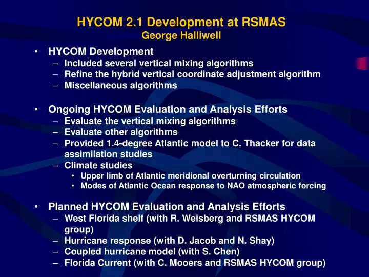
HYCOM 2.1 Development at RSMAS George Halliwell. HYCOM Development Included several vertical mixing algorithms Refine the hybrid vertical coordinate adjustment algorithm Miscellaneous algorithms Ongoing HYCOM Evaluation and Analysis Efforts Evaluate the vertical mixing algorithms

E N D
HYCOM 2.1 Development at RSMASGeorge Halliwell • HYCOM Development • Included several vertical mixing algorithms • Refine the hybrid vertical coordinate adjustment algorithm • Miscellaneous algorithms • Ongoing HYCOM Evaluation and Analysis Efforts • Evaluate the vertical mixing algorithms • Evaluate other algorithms • Provided 1.4-degree Atlantic model to C. Thacker for data assimilation studies • Climate studies • Upper limb of Atlantic meridional overturning circulation • Modes of Atlantic Ocean response to NAO atmospheric forcing • Planned HYCOM Evaluation and Analysis Efforts • West Florida shelf (with R. Weisberg and RSMAS HYCOM group) • Hurricane response (with D. Jacob and N. Shay) • Coupled hurricane model (with S. Chen) • Florida Current (with C. Mooers and RSMAS HYCOM group)
Vertical Mixing Choices in HYCOM 2.1 • Vertical Mixing Models (surface to bottom) • KPP • Mellor-Yamada level 2.5 turbulence closure • Mixed Layer Models • Kraus-Turner A (hybrid) • Kraus-Turner B (hybrid, simplified, from Bleck global HYCOM) • Kraus-Turner C (MICOM mode, from MICOM 2.8) • Price-Weller-Pinkel dynamical instability model • Interior Diapycnal Mixing Models (for use with the mixed layer models) • Explicit algorithm A (hybrid, MICOM-like) • Explicit algorithm B (MICOM mode, from MICOM 2.8) • Implicit algorithm (hybrid, KPP without surface b.l. model)
HYCOM Atlantic Ocean Simulations • Domain • Atlantic Ocean, 20S to 62N • Resolution: 2.0 degrees horizontal, 22 layers vertical • Forcing / Boundary Conditions / Initial Conditions • Surface forcing by COADS climatology • Relaxation to Levitus climatology at N/S boundaries • Relaxation to Levitus surface salinity • Initialized from p(latitude) • Model Runs • 30-year spinup • One-year analysis run • Winter (mid-February) and summer (mid-August) fields saved • Eight Cases Summarized Here to Illustrate Different Vertical Mixing Choices
Latitude Latitude Winter and summer cross-sections along 29W. The central sigma-0 value in the alternating white and gray bands of the shading bar are the isopycnic reference values. Some of the layer numbers are shown inside the shading bar. The thick line is the diagnosed mixed layer base.
Winter mixed layer thickness (m). Experiments: KPP (k-profile parameterization) MY (Mellor-Yamada 2.5) PWP (Price-Weller-Pinkel) KTAI (K-T A m.l., implicit diap.mix.) KTAIP (same with penetrating sw. rad.) KTAE (K-T A m.l., explicit diap. mix.) KTB (K-T B m.l., implicit diap. mix.) MIC (K-T C m.l., MICOM mode)
Winter barotropic stream- function (Sv) Experiments: KPP (k-profile parameterization) MY (Mellor-Yamada 2.5) PWP (Price-Weller-Pinkel) KTAI (K-T A m.l., implicit diap.mix.) KTAIP (same with penetrating sw. rad.) KTAE (K-T A m.l., explicit diap. mix.) KTB (K-T B m.l., implicit diap. mix.) MIC (K-T C m.l., MICOM mode)
Ekman spirals produced by the KPP and MY mixing models in the Westerlies (top) and the trade Winds (bottom). Produced from 32-layer exp- eriments
Winter SST (C) for the KPP experiment (top left). Otherwise, differences between the other seven experiments and the KPP experiment) Experiments: KPP (k-profile parameterization) MY (Mellor-Yamada 2.5) PWP (Price-Weller-Pinkel) KTAI (K-T A m.l., implicit diap.mix.) KTAIP (same with penetrating sw. rad.) KTAE (K-T A m.l., explicit diap. mix.) KTB (K-T B m.l., implicit diap. mix.) MIC (K-T C m.l., MICOM mode)
Summer SST (C) for the KPP experiment (top left). Otherwise, differences between the other seven experiments and the KPP experiment) Experiments: KPP (k-profile parameterization) MY (Mellor-Yamada 2.5) PWP (Price-Weller-Pinkel) KTAI (K-T A m.l., implicit diap.mix.) KTAIP (same with penetrating sw. rad.) KTAE (K-T A m.l., explicit diap. mix.) KTB (K-T B m.l., implicit diap. mix.) MIC (K-T C m.l., MICOM mode)
Winter SSH (m) for the KPP experiment (top left). Otherwise, differences between the other seven experiments and the KPP experiment) Experiments: KPP (k-profile parameterization) MY (Mellor-Yamada 2.5) PWP (Price-Weller-Pinkel) KTAI (K-T A m.l., implicit diap.mix.) KTAIP (same with penetrating sw. rad.) KTAE (K-T A m.l., explicit diap. mix.) KTB (K-T B m.l., implicit diap. mix.) MIC (K-T C m.l., MICOM mode)
Winter sigma-0 for the KPP experiment (top left) along A 29W cross-section. Otherwise, differences between the other seven experiments and the KPP experiment) Experiments: KPP (k-profile parameterization) MY (Mellor-Yamada 2.5) PWP (Price-Weller-Pinkel) KTAI (K-T A m.l., implicit diap.mix.) KTAIP (same with penetrating sw. rad.) KTAE (K-T A m.l., explicit diap. mix.) KTB (K-T B m.l., implicit diap. mix.) MIC (K-T C m.l., MICOM mode)
Winter SST differences (C) between the eight experiments and Levitus climatology. Experiments: KPP (k-profile parameterization) MY (Mellor-Yamada 2.5) PWP (Price-Weller-Pinkel) KTAI (K-T A m.l., implicit diap.mix.) KTAIP (same with penetrating sw. rad.) KTAE (K-T A m.l., explicit diap. mix.) KTB (K-T B m.l., implicit diap. mix.) MIC (K-T C m.l., MICOM mode)
Summer SST differences (C) between the eight experiments and Levitus climatology. Experiments: KPP (k-profile parameterization) MY (Mellor-Yamada 2.5) PWP (Price-Weller-Pinkel) KTAI (K-T A m.l., implicit diap.mix.) KTAIP (same with penetrating sw. rad.) KTAE (K-T A m.l., explicit diap. mix.) KTB (K-T B m.l., implicit diap. mix.) MIC (K-T C m.l., MICOM mode)
Winter sigma-0 differences along 29W between the eight experiments and Levitus climatology. Experiments: KPP (k-profile parameterization) MY (Mellor-Yamada 2.5) PWP (Price-Weller-Pinkel) KTAI (K-T A m.l., implicit diap.mix.) KTAIP (same with penetrating sw. rad.) KTAE (K-T A m.l., explicit diap. mix.) KTB (K-T B m.l., implicit diap. mix.) MIC (K-T C m.l., MICOM mode)
Figure: Preliminary simulation for the Gilbert case using HYCOM including three non-slab Schemes: (a) mixed layer depth, (b) mixed layer temperature, (c) zonal current, (d) meridional current, and e) surface fluxes to the atmosphere. The differences in the directly forced region are much larger between these schemes compared to those used in MICOM simulations. A surface flux difference of up to 500 Wm2is seen at the point of closest approach of storm center. Red, Green, Blue and Cyan lines represent quantities simulated using KT, KPP, MY and PWP schemes respectively.