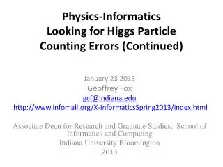
Physics-Informatics Looking for Higgs Particle Counting Errors (Continued)

1. Physics-Informatics Looking for Higgs ParticleCounting Errors (Continued) January 23 2013 Geoffrey Fox gcf@indiana.edu http://www.infomall.org/X-InformaticsSpring2013/index.html Associate Dean for Research and Graduate Studies,  School of Informatics and Computing Indiana University Bloomington 2013

2. Top Topics

3. http://grids.ucs.indiana.edu/ptliupages/publications/Where%20does%20all%20the%20data%20come%20from%20v7.pdhttp://grids.ucs.indiana.edu/ptliupages/publications/Where%20does%20all%20the%20data%20come%20from%20v7.pd This analysis raw data  reconstructed data  AOD and TAGS  Physics is performed on the multi-tier LHC Computing Grid. Note that every event can be analyzed independently so that many events can be processed in parallel with some concentration operations such as those to gather entries in a histogram. This implies that both Grid and Cloud solutions work with this type of data with currently Grids being the only implementation today. ATLAS Expt Note LHC lies in a tunnel 27 kilometres (17 mi) in circumference Higgs Event The LHC produces some 15 petabytes of data per year of all varieties and with the exact value depending on duty factor of accelerator (which is reduced simply to cut electricity cost but also due to malfunction of one or more of the many complex systems) and experiments. The raw data produced by experiments is processed on the LHC Computing Grid, which has some 200,000 Cores arranged in a three level structure. Tier-0 is CERN itself, Tier 1 are national facilities and Tier 2 are regional systems. For example one LHC experiment (CMS) has 7 Tier-1 and 50 Tier-2 facilities.

4. http://www.quantumdiaries.org/2012/09/07/why-particle-detectors-need-a-trigger/atlasmgg/http://www.quantumdiaries.org/2012/09/07/why-particle-detectors-need-a-trigger/atlasmgg/ Model

6. These “Feynman diagrams” define a model. It cannot be calculated exactly but approximate calculations are possible

7. Event Counting • A lot of data analysis consists of setting up a process that gives “events” as a result • Take a survey of what people feel; event is voting of an individual • Build a software system and categorize each of your data; event is this categorization • Sensor Nets; event is result of a sensor measurement • Often results are yes/no • Did person vote for Candidate X or not? • Did event fall into a certain bin of histogram or not? • Note event might have a result (cost of Hotel stay or Mass of Higgs) which is histogrammed; the decision as to which bin to go into is a yes/no decision

8. Generate a Physics Experiment with Python import numpy as np import matplotlib.pyplot as plt testrand = np.random.rand(42000) Base = 110 + 30* np.random.rand(42000) index = (1.0 - 0.5* (Base-110)/30) > testrand gauss = 2 * np.random.randn(300) +126 Sloping = Base[index] NarrowGauss = 0.5 * np.random.randn(300) +126 total = np.concatenate((Sloping, gauss)) NarrowTotal = np.concatenate((Sloping, NarrowGauss))

9. Python Resources • http://www.enthought.com/products/epdgetstart.php Python distribution including NumPy and SciPy with plot package matplotlib • Also pandas and iPython • Python for Data AnalysisAgile Tools for Real World DataByWes McKinney • Publisher: O'Reilly Media • Released: October 2012 • Pages: 472

10. Sloping

11. Sloping 1% Data

12. Higgs on its own

13. Actual Wide Higgs plus Sloping Background

14. Actual Wide Higgs plus Sloping Background with errors

15. Actual Wide Higgs plus Sloping BackgroundData Size divided by 10

16. Narrow Higgs plus Sloping Background2 GeV Bins

17. Narrow Higgs plus Sloping Background1 GeV Bins

18. Narrow Higgs plus Sloping Background0.5 GeV Bins

19. What Happens if more Higgs produced • gaussbig = 2 * np.random.randn(30000) +126 • gaussnarrowbig = 0.5 * np.random.randn(30000) +126 • totalbig = np.concatenate((Sloping, gaussbig))

20. 30,000 Higgs (Real Width and Narrow)

21. 30,000 Higgs (Real Width) + Background

22. Simplification with flat background • import numpy as np • import matplotlib.pyplot as plt • Base = 110 + 30* np.random.rand(42000) • # Base is set of observations with an expected 2800 background events per bin • # Note we assume here flat but in class I used a "sloping" curve that represented experiment better • gauss = 2 * np.random.randn(300) +126 • # Gauss is Number of Higgs particles • simpletotal = np.concatenate((Base, gauss)) • # simpletotal is Higgs+Background • plt.figure("Total Wide Higgs Bin 2 GeV") • values, binedges, junk = plt.hist(simpletotal, bins=15, range =(110,140), alpha = 0.5, color="green") • centers = 0.5*(binedges[1:] + binedges[:-1]) • # centers is center of each bin • # values is number of events in each bin • # :-1 is same as :Largest Index-1 • # binedges[:-1] gets you lower limit of bin • # 1: gives you array starts at second index (labelled 1 as first index 0) • # binedges[1:] is upper limit of each bin • # Note binedges has Number of Bins + 1 entries; centers has Number of Bins entries • errors =sqrt(values) • # errors is expected error for each bin • plt.hist(Base, bins=15, range =(110,140), alpha = 0.5, color="blue") • plt.hist(gauss, bins=15, range =(110,140), alpha = 1.0, color="red") • plt.errorbar(centers, values, yerr = errors, ls='None', marker ='x', color = 'black', markersize= 6.0 )

23. Uniform Background