Download
1 / 14
220 likes | 539 Vues
Monte Carlo Simulation. A technique that helps modelers examine the consequences of continuous risk Most risks in real world generate hundreds of possible outcomes Provides fuller picture of the risk in an asset or investment by considering Different input assumptions & scenarios

E N D
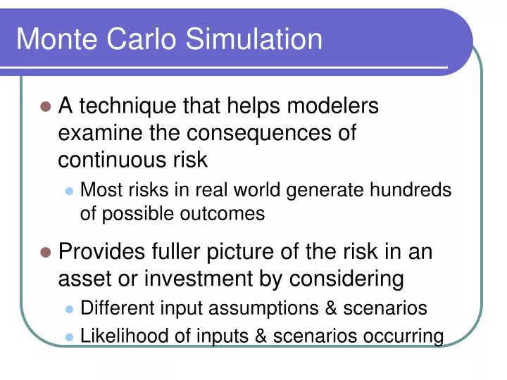
Monte Carlo Simulation • A technique that helps modelers examine the consequences of continuous risk • Most risks in real world generate hundreds of possible outcomes • Provides fuller picture of the risk in an asset or investment by considering • Different input assumptions & scenarios • Likelihood of inputs & scenarios occurring
5 Steps of Monte Carlo Simulation • Build a spreadsheet model that has dynamic relationships between input assumptions and key outputs • Perform sensitivity analysis to identify the key uncertain inputs that have the most potential impact on the key outputs • Quantify possible values for the key uncertain inputs by specifying probability distributions • Simulate numerous scenarios from the input probability distributions and record output results • Summarize recorded output results to measure risks and likelihood of different outcomes
Random Number Generator (RNG) • =Rand() function in Excel • Randomly generates a number between 0 and 1 • Used to represent a cumulative probability P(X) between 0% and 100% • Will be used to identify the input value X such that the probability that value X or a lower value occurs is equal to P(X) • For example, • Rand()=.5 • Used to find input assumption value X where 50% of the input assumption values are smaller and 50% of possible input assumption values are larger than X. • Rand()=.9 • Used to find input assumption value X where 90% of the input assumption values are smaller than X.
Normal (u, σ) P(X≤u)=.5 P(u- σ ≤x ≤u+ σ)=.65 σ Prob u- σ u u+ σ x
Normal Input Distributions • =Norminv(rand(), mean, standard deviation) • For a specified mean and standard deviation, this formula looks up the value for the input distribution that results in rand()% of the assumption values being smaller than the returned value. • The Normal distribution is a continuous distribution
Continuous –vs- Discrete Distributions • In discrete distributions, the values generated for a random variable must be from a finite distinct set of individual values. • In continuous distributions, the values generated for a random variable are specified from a set of uninterrupted values over a range; an infinite number of values is possible
Uniform (a, b) Prob P(X ≤ u)=. 5 a u=a+(b-a) b X 2
Uniform Distribution • =a + (b-a)*rand() • Where a is the smallest value that could occur, b is the largest value • Values between a and b are assumed to be equally likely to occur • Values are assumed to be continuous and not discrete
Triangular Distribution • For symmetrical triangles: • =a + (b-a)*(rand()+rand())/2 • Where a is the smallest value that could occur, b is the largest value • m is the most likely value to occur and is assumed to be halfway between a and b for symmetrical triangles • Values are assumed to be continuous and not discrete in both symmetrical and nonsymmetrical triangular distributions
Discrete Distribution P(x) • XP(x) • .2 • .3 • .4 • .1 10 11 12 13 x
Cumulative Probability Distribution .2 • XP(x) • .2 • .3 • .4 • .1 P(X≤x) .2 .5 .9 1.0 11 10 1.0/0 .5 13 .9 12
Discrete Distributions • Set up a table where the first two columns contain the cumulative probability range for a value and the third column contains the respective discrete values. Make sure the first column starts at 0
Vlookup formula for the Discrete Distribution • Use the Excel function: =vlookup(rand(),table,3) • This function will look up the rand() number in column 1 of the table, identify the row that represents the correct cumulative probability, and look up the value associated with that probability in column 3. • See Vlookup Excel Tutorials in MyLMUConnectfor logic of the Vlookup formula
Specifiying Input Distributions • Practice in Class Exercise 2!