Download
1 / 45
550 likes | 1.14k Vues
Chapter 13 Aggregate Planning. Seasonal variation in demand E.g. Ice Cream Factories Agora on employment and departmental space allocation. Long range. Intermediate range. Short range. Now. 2-3 months. 18 Months. Planning Horizon/Levels.

E N D
Chapter 13Aggregate Planning Seasonal variation in demand E.g. Ice Cream Factories Agora on employment and departmental space allocation
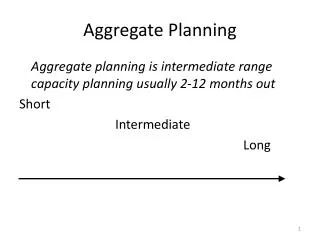
Long range Intermediate range Short range Now 2-3 months 18 Months Planning Horizon/Levels Aggregate planning: Intermediate-range capacity planning, usually covering 2 to 12 months. (Also called Macro planning)
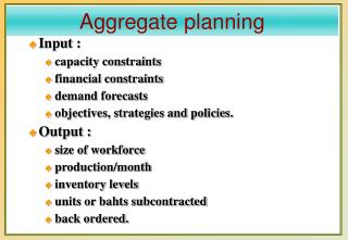
To develop a feasible production plan on an aggregate level that achieves a balance of expected demand and supply usually demand and supply are converted to aggregate units such as labour-hours, working days, general product units, etc. Why do it? Objective of Aggregate Planning
Maintain a level workforce Maintain a steady output rate Match demand period by period Use a combination of decision variables Aggregate Planning Approaches
Demand Demand Demand Level and Chase Strategies Quantity Normal capacity Level Output Strategy Output less than demand Output level Output exceeds demand Chase Demand Strategy Output above normal Normal capacity Output below normal
6 7 1 2 3 4 5 8 9 10 Cumulative Graph Cumulative output/demand Cumulative production Cumulative demand
An NSU UG student One year expenses tuition 40,000 transportation 1000 x 12 = 12000 food and meal 2000 x 10 = 20000 summer 5000 x 2 = 10000 others 500 x 12 = 6000 Total 88,000 Example - a personal plan
A NSU UG student plan income Bank loan, etc 40000 private tutoring 2000 x 12 = 24000 part time job 2000 x 10 = 20000 summer job 6500 x 2 = 13000 family money 1000 x 10 = 10000 Total 107000 saving 107000 - 88000 = 19000 Objective: income meets expenses; maximize saving; etc. (What do you call this?) Example - a personal plan
1. Forecast demand in the period 2. Develop plan(s) to meet the demand by setting levels on output, employment, inventory, etc. 3. The plans are refined or reworked until a feasible and satisfactory plan is uncovered. General steps in AP
Pricing e.g., shift demands from peak periods to off-peak periods. The more the elasticity, the more effective pricing will be on the demand pattern. Promotion Backorders (depend on customers’ willingness) Develop new demand (market) during off-peak period Options to affect demand level
Hire and fire workers - depends on the intensity of labour used, the strength of the union, corporate culture, labour laws, etc. Overtime/slack time - to keep a skilled workforce and allows employee to increase earnings Partime workers - depend on nature of work Inventories - smooth production and buffer against demand surge; could be costly Subcontracting - capacity increase in a short time without heavy investment; less control Options to affect capacity
Linear programming: Methods for obtaining optimal solutions to problems involving allocation of scarce resources in terms of cost minimization. Linear decision rule: Optimizing technique that seeks to minimize combined costs, using a set of cost-approximating functions to obtain a single quadratic equation. Mathematical Techniques
Example The VP of Operations is about to prepare the aggregate plan that will cover six periods in the horizon. The company has forecasted the following demand: The output cost is $2 per unit at regular time; $3 per unit at overtime; $6 per unit if subcontracted. Average inventory cost is $1 per unit per period. Back orders are possible, however, the Company estimated the cost to be $5 per unit per period. The initial inventory is zero. There are 15 workers and each worker is able to produce 20 units of the product per period. Can you help the VP to develop an aggregate plan?
Average inventory Beginning Inventory + Ending Inventory = 2 Example - solution • Suppose the VP wants to use a leveling (capacity) approach, I.e., maintaining a steady rate of output. The total output by the workers at the regular time is 20 x 15 x 6 = 1800 which equals to the forecast demand.
The VP learned that a regular worker is retiring. Rather than hiring new worker, the VP decides to use overtime. However, the maximum amount of overtime output is 40 units per period. Suggest an aggregate plan for the VP Regular worker produce 14 x 20 units = 280 units per period. The total deficiency is 120 units. These 120 units can be satisfied in 3 periods by overtime and can be produced during the periods of high demand (for cost consideration. Of course, you can put them in other periods too.) Example- Chase demand
Quantitative approach Suppose the VP wants to use a more quantitative approach that use overtime only and have in mind that the cost be minimized. Can you help him? Let us define the following notation: Pt = No. of units produced via regular time at period t, t=1, …, 6 Dt= Demand (in No. of units) at period t, t=1, …, 6 Ot= No. of units produced at period t in overtime, t=1, …, 6 It = Inventory level (in No. of units) at the end of period t, t=1, …, 6
For ease of handling, we introduce the concept of back order Bt at period t. The following is a kind of “conservation law” It = It-1 + Pt - Dt , t = 1, …, 6. The Objective function is given by: Notice that I0 = 0 and B0 = 0, (D1, …, D6) = (200,200,300,400,500,200)
The aggregate plan gives the level of demand and supply in aggregate units at the macro level In order for the company to execute the plan, it needs to disaggregate the plan into appropriate units for implementation and monitoring. The output of this process is a master schedule and a master production schedule. Disaggregating the aggregate plan
Master Scheduling Process A master schedule is a schedule (usually in the form of a table) indicating the quantity and timing (I.e., delivery times) for individual products or a group of individual products. Inputs Outputs
Beginning Inventory Forecast is larger than Customer orders in week 3 Customer orders are larger than forecast in week 1 Forecast is larger than Customer orders in week 2 Projected On-hand Inventory Figure 13.8
Suppliments Relevant important ideas
Services generally have variable processing requirements that make it difficult to establish a suitable measure of capacity. Capacity availability can be difficult to predict Services occur when they are rendered. Services cannot be stockpiled or inventoried so they do not have this option. It is considered "perishable,“ An empty hotel room cannot be held and sold later Demand for service can be difficult to predict Labor flexibility can be an advantage in services Aggregate Planning in Services
Time Fences in MPS • Time Fences – points in time that separate phases of a master schedule planning horizon. Period “frozen”(firm orfixed) “liquid”(open) “slushy”somewhatfirm
Calculated only in current week and any week with MPS>0 Current period: on-hand plus any current period MPS, minus all orders in that and subsequent periods until next MPS Later periods: MPS – all orders until next MPS Calculating ATP
level production plan Different sales forecast - Same total: 120 units, starts lower, goes higher
“Chase” production strategy Production adjusts to meet demand
Lot size of 30 units Produce if projected balance falls below 5 units Extra on-hand inventory is “cycle stock” 5 unit “trigger” is safety stock
Indented BOM Bike Frame Assembly Components Frame Wheel Assembly Wheel Hubs & Rims Spokes Tires BOM formats • Single-level BOM only shows one layer down. Wheel Assembly Wheel Tires
Low-Level Code Numbers • Lowest level in structure item occurs • Top level is 0; next level is 1 etc. • Process 0s first, then 1s • Know all demand for an item • Where should blue be? LLC 0 1 2 3 4 The low-level code controls the sequence in which the materialis planned in an MRP run: First the materials with low-level code 0 areplanned, then the materials with low-level code 1, and so on. The lowerthe low-level code, the higher the number that is assigned to thematerial.
LLC Drawing • Item only appears in one level of LLC drawing • Easier to understand • Simplifies calculations LLC 0 1 2 3 4
Master Production schedule is anticipated build schedule FAS is actual build schedule Exact end-item configurations Final Assembly Schedule
Stable schedule means stable component schedules, more efficient No changes means lost sales Frozen zone- no changes at all Time fences >24 wks, all changes allowed (water) 16-23 wks substitutions, if parts there (slush) 8-16 minor changes only (slush) < 8 no changes (ice) Schedule Stability