Chapter 4. Continuous Random Variables and Probability Distributions

Chapter 4. Continuous Random Variables and Probability Distributions Weiqi Luo (骆伟祺) School of Software Sun Yat-Sen University Email：weiqi.luo@yahoo.com Office：# A313

Chapter four: Continuous Random Variables and Probability Distributions • 4.1 Continuous Random Variables and Probability Density Functions • 4.2 Cumulative Distribution Functions and Expected Values • 4.3 The Normal Distribution • 4.4 The Gamma Distribution and Its Relatives • 4.5 Other Continuous Distributions • 4.6 Probability Plots

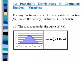
4.1 Continuous Random Variables and Probability Density Functions • Continuous Random Variables A random variable X is said to be continuous if its set of possible values is an entire interval of numbers – that is , if for some A<B, any number x between A and B is possible

4.1 Continuous Random Variables and Probability Density Functions • Example 4.2 If a chemical compound is randomly selected and its PH X is determined, then X is a continuous rv because any PH value between 0 and 14 is possible. If more is know about the compound selected for analysis, then the set of possible values might be a subinterval of [0, 14], such as 5.5 ≤ x ≤ 6.5, but X would still be continuous. 0 14 5.5 6.5

4.1(a) 4.1(c) 4.1 Continuous Random Variables and Probability Density Functions • Probability Distribution for Continuous Variables Suppose the variable X of interest is the depth of a lake at a randomly chosen point on the surface. Let M be the maximum depth, so that any number in the interval [0,M] is a possible value of X. 0 M 0 M 0 M Measured by meter Measured by centimeter A limit of a sequence of discrete histogram Discrete Cases Continuous Case 4.1(b)

f(x) x a b 4.1 Continuous Random Variables and Probability Density Functions • Probability Distribution Let X be a continuous rv. Then a probability distribution or probability density function (pdf) of X is f(x) such that for any two numbers a and b with a ≤ b The probability that X takes on a value in the interval [a,b] is the area under the graph of the density function as follows.

f(x) x a b 4.1 Continuous Random Variables and Probability Density Functions • A legitimate pdf should satisfy

4.1 Continuous Random Variables and Probability Density Functions • pmf (Discrete) vs. pdf (Continuous) p(x) f(x) P(X=c) = p(c) P(X=c) = f(c) ? 0 M 0 M

4.1 Continuous Random Variables and Probability Density Functions • Proposition If X is a continuous rv, then for any number c, P(X=c)=0. Furthermore, for any two numbers a and b with a<b, P(a≤X ≤b) = P(a<X ≤b) = P(a ≤X<b) = P(a <X<b) Impossible event :the event contain no simple element P(A)=0  A is an impossible event ?

4.1 Continuous Random Variables and Probability Density Functions • Uniform Distribution A continuous rv X is said to have a uniform distribution on the interval [A, B] if the pdf of X is

4.1 Continuous Random Variables and Probability Density Functions • Example 4.3 The direction of an imperfection with respect to a reference line on a circular object such as a tire, brake rotor, or flywheel is, in general, subject to uncertainty. Consider the reference line connecting the valve stem on a tire to the center point, and let X be the angle measured clockwise to the location of an imperfection, One possible pdf for X is

f(x) 180 360 4.1 Continuous Random Variables and Probability Density Functions • Example 4.3 (Cont’) 90

4.1 Continuous Random Variables and Probability Density Functions • Example 4.4 “Time headway” in traffic flow is the elapsed time between the time that one car finishes passing a fixed point and the instant that the next car begins to pass that point. Let X = the time headway for two randomly chosen consecutive cars on a freeway during a period of heavy flow. The following pdf of X is essentially the one suggested in “The Statistical Properties of Freeway Traffic”.

4.1 Continuous Random Variables and Probability Density Functions • Example 4.4 (Cont’) 1. f(x) ≥ 0; 2. to show , we use the result

4.1 Continuous Random Variables and Probability Density Functions • Example 4.4 (Cont’) f(x) 0.15 x 2 4 6 8 10 0.5

4.1 Continuous Random Variables and Probability Density Functions • Homework Ex. 2, Ex. 5, Ex. 8

f(x) F(x) F(8) F(8) 0.5 x 5 10 x 8 5 10 4.2 Cumulative Distribution Functions and Expected Values • Cumulative Distribution Function The cumulative distribution function F(x) for a continuous rv X is defined for every number x by For each x, F(x) is the area under the density curve to the left of x as follows 1 8

f(x) f(x) A B x x A B 4.2 Cumulative Distribution Functions and Expected Values • Example 4.5 Let X, the thickness of a certain metal sheet, have a uniform distribution on [A, B]. The density function is shown as follows. For x < A, F(x) = 0, since there is no area under the graph of the density function to the left of such an x. For x ≥ B, F(x) = 1, since all the area is accumulated to the left of such an x.

F(x) 1 A B x 4.2 Cumulative Distribution Functions and Expected Values • Example 4.5 (Cont’) For A ≤X≤ B Therefore, the entire cdf is

f(x) - = a b b a 4.2 Cumulative Distribution Functions and Expected Values • Using F(x) to compute probabilities Let X be a continuous rv with pdf f(x) and cdf F(x). Then for any number a and for any two numbers a and b with a<b

4.2 Cumulative Distribution Functions and Expected Values • Example 4.6 Suppose the pdf of the magnitude X of a dynamic load on a bridge is given by For any number x between 0 and 2, thus

4.2 Cumulative Distribution Functions and Expected Values • Example 4.6 (Cont’) f(x) F(x) 1 7/8 1/8 0 2 2

4.2 Cumulative Distribution Functions and Expected Values • Obtaining f(x) form F(x) If X is a continuous rv with pdf f(x) and cdf F(x), then at every x at which the derivative F’(x) exists, F’(x)=f(x)

4.2 Cumulative Distribution Functions and Expected Values • Example 4.7 (Ex. 4.5 Cont’) When X has a uniform distribution, F(x) is differentiable except at x=A and x=B, where the graph of F(x) has sharp corners. Since F(x)=0 for x<A and F(x)=1 for x>B, F’(x)=0=f(x) for such x. For A<x<B

f(x) 4.2 Cumulative Distribution Functions and Expected Values • Percentiles of a Continuous Distribution Let p be a number between 0 and 1. The (100p)th percentile of the distribution of a continuous rv X , denoted by η(p), is defined by F(x) 1 Shaded area=p

4.2 Cumulative Distribution Functions and Expected Values • Example 4.8 The distribution of the amount of gravel (in tons) sold by a particular construction supply company in a given week is a continuous rv X with pdf The cdf of sales for any x between 0 and 1 is

F(x) 1 .5 x 0 0.347 1 4.2 Cumulative Distribution Functions and Expected Values • Example 4.8 (Cont’)

4.2 Cumulative Distribution Functions and Expected Values • The median The median of a continuous distribution, denoted by , is the 50th percentile, so satisfies 0.5=F( ), that is, half the area under the density curve is to the left of and half is to the right of Symmetric Distribution

4.2 Cumulative Distribution Functions and Expected Values • Expected/Mean Value The expected/mean value of a continuous rv X with pdf f(x) is Discrete Case

4.2 Cumulative Distribution Functions and Expected Values • Example 4.9 (Ex. 4.8 Cont’) The pdf of weekly gravel sales X was So

4.2 Cumulative Distribution Functions and Expected Values • Expected value of a function If X is a continuous rv with pdf f(x) and h(X) is any function of X, then Discrete Case

4.2 Cumulative Distribution Functions and Expected Values • Example 4.10 Two species are competing in a region for control of a limited amount of a certain resource. Let X = the proportion of the resource controlled by species 1 and suppose X has pdf which is a uniform distribution on [0,1]. Then the species that controls the majority of this resource controls the amount The expected amount controlled by the species having majority control is then

4.2 Cumulative Distribution Functions and Expected Values • The Variance The variance of a continuous random variable X with pdf f(x) and mean value μ is The standard deviation (SD) of X is

4.2 Cumulative Distribution Functions and Expected Values • Proposition The Same Properties as Discrete Cases

4.2 Cumulative Distribution Functions and Expected Values • Homework Ex. 12, Ex. 18, Ex. 22, Ex. 23

4.3 The Normal Distribution • Normal (Gaussian) Distribution A continuous rv X is said to have a normal distributionwith parameters μ and σ (or μ and σ2), where -∞ < μ < +∞ and 0 < σ, if the pdf of X is • Note: • The normal distribution is the most important one in all of probability and statistics. Many numerical populations have distributions that can be fit very closely by an appropriate normal curve. • Even when the underlying distribution is discrete, the normal curve often gives an excellent approximation. • Central Limit Theorem (see next Chapter)

4.3 The Normal Distribution • Properties of f(x;μ,σ) Proof? E(X) = μ & V(X) = σ2 , X~ N(μ, σ2 ) σ is large σ is medium σis small Symmetry Shape

4.3 The Normal Distribution • Standard Normal Distribution The normal distribution with parameter values μ=0 and σ=1 is called the standard normal distribution. A random variable that has a standard normal distribution is called a standard normal random variable and will be denoted by Z. The pdf of Z is The cdf of Z is Shaded area= f(z;0,1) 0 z Refer to Appendix Table A.3

4.3 The Normal Distribution • Properties of Φ(z)

4.3 The Normal Distribution • Example 4.12 (a) P(Z≤1.25) (b) P(Z>1.25) (c) P(Z ≤-1.25) Shaded area= z curve Shaded area= 0 1.25 0 0 -1.25 1.25

- = -0.38 0 1.25 0 -0.38 0 1.25 4.3 The Normal Distribution • Example 4.12 (Cont’) (d) P(-0.38 ≤ Z ≤ 1.25)

z curve 0 Percentile (tail area) 90 95 97.5 99 99.5 99.9 99.95 0.1 0.05 0.025 0.01 0.005 0.001 0.0005 1.28 1.645 1.96 2.33 2.58 3.08 3.27 4.3 The Normal Distribution • zαnotation zα will denote the values on the measurement axis for which α of the area under the z curve lies to the right of zα Shaded area=P(Z≥ zα)=α Note: Zαis the 100(1- α)th percentile of the standard normal distribution

4.3 The Normal Distribution • Nonstandard Normal Distribution If X has the normal distribution with mean μ and standard deviation σ, then has a standard normal distribution (why?).Thus

4.3 The Normal Distribution • Equality of nonstandard and standard normal curve area σ =1 x (x- μ)/ σ Percentiles of an Arbitrary Normal Distribution Refer to Ex. 4.17

4.3 The Normal Distribution • Example 4.15 The time that it takes a driver to react to the brake lights on a decelerating vehicle is critical in helping to avoid rear-end collisions . Reaction time for an in-traffic response to a brake signal from standard brake lights can be modeled with a normal distribution having mean value 1.25 sec and standard deviation of .46 sec . What is the probability that reaction time is between 1.00 sec and 1.75 sec?

4.3 The Normal Distribution • Example 4.16 The breakdown voltage of a randomly chosen diode of a particular type is known to be normally distributed. What is the probability that a diode’s breakdown voltage is within 1 standard deviation of its mean value? Note: This question can be answered without knowing either μ or σ, as long as the distribution is known to be normal; in other words , the answer is the same for any normal distribution:

4.3 The Normal Distribution • If the population distribution of a variable is (approximately) normal, then • Roughly 68% of the values are within 1 SD of the mean. • Roughly 95% of the values are within 2 SDs of the mean • Roughly 99.7% of the values are within 3 SDs of the mean 99.7% 95% 68% μ-2σ μ+2σ μ+3σ μ-1σ μ-3σ μ+1σ

4.3 The Normal Distribution • The Normal Distribution and Discrete Populations Ex. 4.18: IQ in a particular population is known to be approximately normally distributed with μ = 100 and σ = 15. What is the probability that a randomly selected individual has an IQ of at least 125? Letting X = the IQ of a randomly chosen person, we wish P(X ≥125). The temptation here is to standardize X ≥ 125 immediately as in previous example. However, the IQ population is actually discrete, since IQs are integer-valued, so the normal curve is an approximation to a discrete probability histogram, continuity correction … ≠ 0 125 124.5 125.5

4.3 The Normal Distribution • The Normal Approximation to the Binomial Distribution Recall that the mean value and standard deviation of a binomial random variable X are μX = np and σX=(npq)1/2. Consider the binomial probability histogram with n = 20, p = 0.6. It can be approximated by the normal curve with μ = 12 and σ = 2.19 as follows. 0.20 Normal curve A bit skewed (p ≠ 0.5) 0.15 0.10 0.05 0 2 4 6 8 10 12 14 16 18 20

4.3 The Normal Distribution • Proposition Let X be a binominal rv based on n trials with success probability p. Then if the binomial probability histogram is not too skewed, X has approximately a normal distribution with μ = np and σX=(npq)1/2. In particular, for x = a possible value of X , Rule: In practice, the approximation is adequate provided that both np≥10 and nq ≥10. (where q=1-p)

Chapter 4. Continuous Random Variables and Probability Distributions