Download

1 / 35
390 likes | 797 Vues
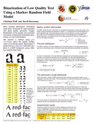
Markov random field: A brief introduction. Tzu-Cheng Jen Institute of Electronics, NCTU 2007-03-28. Outline. Neighborhood system and cliques Markov random field Optimization-based vision problem Solver for the optimization problem. Neighborhood system and cliques. Prior knowledge.

E N D
Markov random field: A brief introduction Tzu-Cheng Jen Institute of Electronics, NCTU 2007-03-28
Outline • Neighborhood system and cliques • Markov random field • Optimization-based vision problem • Solver for the optimization problem
Prior knowledge • In order to explain the concept of the MRF, we first introduce following definition: 1. i: Site (Pixel) 2. Ni: The neighboring point of i 3. S: Set of sites (Image) 4. fi: The value at site i (Intensity) A 3x3 imagined image
Neighborhood system • The sites in S are related to one another via a neighborhood system. Its definition for S is defined as: where Ni is the set of sites neighboring i. • The neighboring relationship has the following properties: (1) A site is not neighboring to itself (2) The neighboring relationship is mutual
Neighborhood system: Example First order neighborhood system Second order neighborhood system Nth order neighborhood system
Neighborhood system: Example The neighboring sites of the site i are m, n, and f. The neighboring sites of the site j are r and x
Clique • A clique C is defined as a subset of sites in S. Following are some examples
Clique: Example • Take first order neighborhood system and second order neighborhood for example: Neighborhood system Clique types
Markov random field (MRF) • View the 2D image f as the collection of the random variables (Random field) • A random field is said to be Markov random field if it satisfies following properties Image configuration f
Gibbs random field (GRF) and Gibbs distribution • A random field is said to be a Gibbs random field if and only if its configuration f obeys Gibbs distribution, that is: Design U for different applications Image configuration f U(f): Energy function; T: Temperature Vi(f): Clique potential
Markov-Gibbs equivalence • Hammersley-Clifford theorem: A random field F is an MRF if and only if F is a GRF Proof(<=): Let P(f) be a Gibbs distribution on S with the neighborhood system N. A 3x3 imagined image
Markov-Gibbs equivalence • Divide C into two set A and B with A consisting of cliques containing i and B cliques not containing i: A 3x3 imagined image
Denoising Noisy signal d denoised signal f
MAP formulation for denoising problem • The problem of the signal denoising could be modeled as the MAP estimation problem, that is, (Observation model) (Prior model)
MAP formulation for denoising problem • Assume the observation is the true signal plus the independent Gaussian noise, that is • Under above circumstance, the observation model could be expressed as U(d|f): Likelihood energy
MAP formulation for denoising problem • Assume the unknown data f is MRF, the prior model is: • Based on above information, the posteriori probability becomes
MAP formulation for denoising problem • The MAP estimator for the problem is: ?
MAP formulation for denoising problem • Define the smoothness prior: • Substitute above information into the MAP estimator, we could get: Observation model (Similarity measure) Prior model (Reconstruction constrain)
Super-resolution • Super-Resolution (SR): A method to reconstruct high-resolution images/videos from low-resolution images/videos
Super-resolution • Illustration for super-resolution d(1) d(2) d(3) d(4) Use the low-resolution frames to reconstruct the high resolution frame f(1)
MAP formulation for super-resolution problem • The problem of the super-resolution could be modeled as the MAP estimation problem, that is, (Observation model) (Prior model)
MAP formulation for super-resolution problem • The conditional PDF can be modeled as the Gaussian distribution if the noise source is Gaussian noise • We also assume the prior model is joint Gaussian distribution
MAP formulation for super-resolution problem • Substitute above relation into the MAP estimator, we can get following expression: (Observation model) (Prior model)
The solver of the optimization problem • In this section, we will introduce different approaches for solving the optimization problem: 1. Brute-force search (Global extreme) 2. Gradient descent search (Local extreme, Usually) 3. Genetic algorithm (Global extreme) 4. Simulated annealing algorithm (Global extreme)
Simulation: SR by gradient descent algorithm Use 6 low resolution frames (a)~(f) to reconstruct the high resolution frame (g)
The problem of the gradient descent algorithm • Gradient descent algorithm may be trapped into the local extreme instead of the global extreme
Genetic algorithm (GA) • The GA includes following steps:
Simulated annealing (SA) • The SA includes following steps: