Download
1 / 1
10 likes | 89 Vues
Application and Refinement of a Method to Achieve Uniform Convective Response on Variable-Resolution Meshes Robert L. Walko 1 , David Medvigy 2 , and Roni Avissar 1

E N D
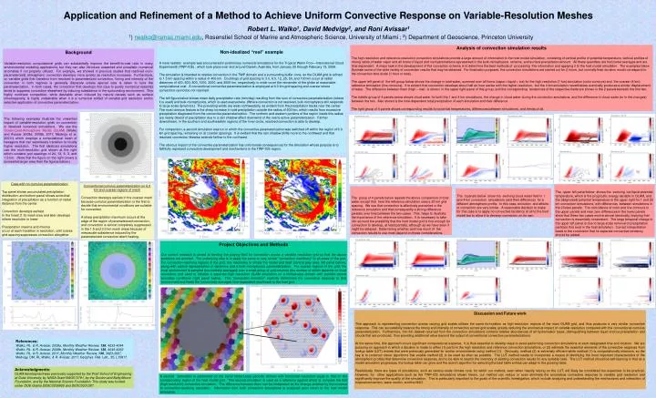
Application and Refinement of a Method to Achieve Uniform Convective Response on Variable-Resolution Meshes Robert L. Walko1, David Medvigy2, and Roni Avissar1 1) rwalko@rsmas.miami.edu, Rosenstiel School of Marine and Atmospheric Science, University of Miami; 2) Department of Geoscience, Princeton University Analysis of convection simulation results The high resolution and reference-resolution convection simulations provide a large amount of information to the host model simulation, consisting of vertical profile of potential temperature, vertical profiles of mixing ratios of water vapor and all forms of liquid and ice hydrometeors represented in the bulk microphysics scheme, and surface precipitation amount. All these quantities are horizontal averages and are time dependent. A major task in the development of this convection scheme is to determine the best methods of processing this information and applying it to the host model simulation. The examples below illustrate some of the wide variety of convection results that may be obtained. For illustration purposes, the convection simulations are carried out for 2 hours, but normally their duration would correspond to the convection time scale (1 hour or less). The upper left panel of the left group below shows the change in total water, summed over all forms (vapor+ liquid + ice) for the high resolution (1 km) simulation (color contours) and the coarser (4 km) reference simulation (line contours). It is evident that convection develops about half an hour earlier with the higher resolution, but the 4 km simulation nevertheless eventually produces a similar displacement of water. The difference between them (high – low) is shown in the upper right panel of this group, and the corresponding tendencies of the respective fields are shown in the 2 panels beneath the first two. The middle group of 4 panels below shows cloud water for both the 1 and 4 km simulations, the change in cloud water during the convection simulations, and the difference in cloud water (or in the changes) between the two. Also shown is the time-dependent total precipitation of each simulation and their difference. The right group of 4 panels shows corresponding results for potential temperatures, differences between simulations, and trends of all. Non-idealized “real” example A more realistic example was encountered in preliminary numerical simulations for the Tropical Warm Pool—International Cloud Experiment6 (TWP-ICE) , which took place over and around Darwin, Australia, from January 20 through February 13, 2006. The simulation is intended to resolve convection in the TWP domain and a surrounding buffer cone, so the OLAM grid is refined to 1.5 km spacing within a radius of 400 km. Doublings of grid spacing to 3.0, 6.0, 12, 25, 50, and 100 km occur at radial distances of 400, 600, 800, 1000, 2000, and 3000 km, respectively, in order cover the remainder of the globe at reasonable computational cost. A conventional convective parameterization is employed at 6.0 km grid spacing and coarser where convection cannot be not resolved. The left figure below shows mean daily precipitation rate (mm/day) resulting from the sum of convective parameterization (where it is used) and bulk microphysics, which is used everywhere. (Where convection is not resolved, bulk microphysics still responds to large-scale dynamics.) The prevailing winds are west-northwesterly, as evident from the precipitation tracks near the center. The most obvious feature is the sharp increase in total precipitation outside the radius of 600 km, which results from excessive precipitation diagnosed from the convective parameterization. The northern and western portions of the region inside this radius are nearly devoid of precipitation due to a rain shadow effect downwind of the overly-active parameterization. Farther downstream, in the southern and southeastern regions of the inner circle, resolved convection is able to develop. For comparison, a second simulation was run in which the convective parameterization was switched off within the region of 6.0 km grid spacing, remaining on at coarser spacings. It is evident that the rain shadow shifts more to the northwest and that resolved convection likewise extends farther to the northwest. The obvious impact of the convective parameterization has unfortunate consequences for the simulation whose purpose is to faithfully represent convective development and mechanisms in the TWP-ICE region. Background Variable-resolution computational grids can substantially improve the benefit-to-cost ratio in many environmental modeling applications, but they can also introduce unwanted and unrealistic numerical anomalies if not properly utilized. For example, we showed in previous studies that resolved (non-parameterized) atmospheric convection develops more quickly as resolution increases. Furthermore, on variable grids that transition from resolved to parameterized convection, timing and intensity of the convection in both regimes is generally disparate unless special care is taken to tune the parameterization. In both cases, the convection that develops first (due to purely numerical reasons) tends to suppress convection elsewhere by inducing subsidence in the surrounding environment. This highly nonlinear competition, while desirable when induced by natural causes such as surface inhomogeneity, is highly undesirable when it is a numerical artifact of variable grid resolution and/or selective application of convective parameterization. The following examples illustrate the unwanted impact of variable-resolution grids on convection in idealized numerical simulations. We use the Ocean-Land-Atmosphere Model (OLAM) (Walko and Avissar 2008a, 2008b, 2011; Medvigy et al. 20011) which employs a computational mesh of hexagons that can seamlessly transition to locally higher resolution. The first idealized simulations use the multi-resolution grid shown at the right which contains grid spacings of 24, 12, 6, 3, and 1.5 km. (Note that the figure on the right covers a somewhat larger area than the figures below.) Case with no cumulus parameterization Top panel shows accumulated precipitation distribution, and bottom panel shows azimuthal integration of precipitation as a function of radial distance from the center. Convection develops earliest In the finest (1.5) mesh area and later develops where resolution is lower. Precipitation maxima and minima occur at each transition in resolution, until coarse grid spacing suppresses convection altogether. Conventional cumulus parameterization on 6.0 km and coarser regions of mesh Convection develops earliest in the coarser mesh because cumulus parameterization is the first to decide that environmental conditions are suitable for convection. A sharp precipitation maximum occurs at the edge of the region of parameterized convection, and convection is almost completely suppressed in the 1.5 and 3.0 km mesh areas because of mesoscale subsidence induced by the parameterized convective latent heating. The upper left panel below shows the evolving ice-liquid potential temperature, which is the prognostic energy variable in OLAM, and the (diagnosed) potential temperature in the upper right for 1 and 20 km convection simulations, with differences between simulations in the 2 lower panels. The coincidence of color and line contours in the upper panels and near zero differences in the lower panels show that these two cases evolve almost identically, implying that convection is essentially nonexistent. The large temporal change in the upper left panel is due to large-scale removal of precipitation particles that exist in the host simulation. Correct interpretation leads to the conclusion that no separate convective tendency should be added. The group of 4 panels below repeats the above comparison of total water except that here the reference simulation uses a 20 km grid spacing. We see that convection is effectively prevented in the reference simulation and that consequently a strong difference persists over time between the two cases. This helps to illustrate the importance of the reference simulation: It is necessary to take into account the possibility that the host model grid is fine enough for convection to develop, at least partially, although as we have seen it might be delayed. Determining whether and how much of the convection results to use must depend on these considerations. The 3 panels below show the evolving cloud water field in 1 and 4 km convection simulations (and their difference) for a different atmospheric profile. In this case, evolution and effects of convection are very similar. A reasonable decision to make for this case is to apply no convective tendency at all to the host model but to allow it to develop convection on its own. theta_223HL Project Objectives and Methods Our current research is aimed at leveling the playing field for convection across a variable resolution grid so that the above problems are avoided. The underlying idea is to apply the same or very similar “convective machinery” to all areas of the grid. For convection-resolving regions of the grid, this machinery is simply the model grid itself (central gray area, left panel below), along with explicit representation of dynamics and a bulk microphysics parameterization. For coarser regions of the grid, the local environment is sampled (horizontally averaged) over a small group of grid columns (the number of which depends on local resolution) and used to initialize a separate high resolution OLAM simulation on a limited-area domain with periodic lateral boundary conditions (right panel below). This “convection simulator” explicitly determines the convective response to that environment and feeds the horizontally-averaged time-dependent result back to the host grid. Discussion and Future work This approach to representing convection across varying grid scales utilizes the same formulation as high-resolution regions of the main OLAM grid, and thus produces a very similar convective response. This can successfully balance the timing and intensity of convection across grid scales, greatly reducing the anomalous impact of variable resolution compared with the conventional cumulus parameterization. Furthermore, the rich dataset returned from the convection simulations contains relative abundances of all hydrometeor types, distinguishing between liquid and ice precipitation and clouds that are produced, thus providing additional value beyond the output of conventional convective parameterizations. At the same time, this approach incurs significant computational expense. It is thus essential to develop ways to avoid performing convection simulations at each designated time and location. We are pursuing an approach in which a decision is made to either (1) perform the high resolution and reference convection simulations, or (2) estimate the essential elements of the convective response from lookup table (LUT) entries that were previously generated for similar environments using method (1). Obviously, method (2) is extremely efficient while method (1) is computationally intensive, so the key is to construct clever algorithms that enable method (2) to be used as often as possible. The LUT method needs to incorporate a means of identifying the most important characteristics of the atmospheric profiles that determine convective response, and to be able to search the inventory of existing convection results for any suitable case. The LUT method should be self-learning in that as a model simulation progresses, the lookup table can grow and the search algorithm for selecting the best table entries can adapt to the growing table. Realistically, there are types of simulations, such as century-scale climate runs, for which our method, even when heavily relying on the LUT, will likely be considered too expensive to be practical. However, for other applications such as the TWP-ICE simulations shown herein, our method can reduce or even eliminate the anomalous convective response to variable grid resolution and significantly improve the quality of the simulation. This is particularly important to the goals of the scientific investigation, which include analyzing and understanding the mechanisms and interaction of tropical convection, wave motion, and the MJO. References: Walko, RL. & R. Avissar, 2008a, Monthly Weather Review, 136, 4033-4044 Walko, RL. & R. Avissar, 2008b, Monthly Weather Review, 136, 4045-4062 Walko, RL. & R. Avissar, 2011, Monthly Weather Review, 139, 3923-3937. Medvigy, DM, RL Walko, & R. Avissar, 2011, Geophys. Res. Lett., 35, L15817. Acknowledgments: OLAM development was previously supported by the Pratt School of Engineering at Duke University, by NASA Grant NAG513781, by the Gordon and Betty Moore Foundation, and by the National Science Foundation. This study was funded under DOE Grants DESC0006805 and DESC0001287. A second simulation is performed on the same limited-area periodic domain with horizontal resolution equal to that on the corresponding region of the host model grid. This second simulation is used as a reference against which to compare the first (high resolution) convection simulation. The difference between them can be interpreted as the change enabled by the increase to convection-resolving resolution. Information from both convection simulations is analyzed upon return to the host model simulation.