Download
1 / 52
570 likes | 925 Vues
ADAPTIVE FILTERS FOR REMOVAL OF INTERFERENCE. 2004235124 김현일. 목차. Adaptive Filter Overview Adaptive Noise Cancellor The Least Mean Squares Adaptive Filter The Recursive Least Squares Adaptive Filter Selecting An Appropriate Filter Application : Removal of Artifacts in the ECG

E N D
ADAPTIVE FILTERS FOR REMOVAL OF INTERFERENCE 2004235124 김현일
목차 • Adaptive Filter Overview • Adaptive Noise Cancellor • The Least Mean Squares Adaptive Filter • The Recursive Least Squares Adaptive Filter • Selecting An Appropriate Filter • Application : Removal of Artifacts in the ECG • Application : Adaptive Cancellation of the Maternal ECG to obtain the Fetal ECG • Application : Adaptive Cancellation of Muscle-Contraction Interference in Knee-Joint Vibration Signals 생체 신호 해석
Adaptive Filter Overview (1) • Signal and noise are stationary → Filter with fixed tap weights or coefficients • Frequency filter not suitable when signal/noise vary with time or signal and interference overlap. • Ex ECG signals of a fetus and the mother 생체 신호 해석
Adaptive Filter Overview (2) • Fixed filtering cannot separate them. • Such a situation calls for the use of a filter that can learn and adapt. This requires the filter to automatically adjust its impulse response as the characteristics of the signal and/of noise vary. 생체 신호 해석
The adaptive noise canceller (1) • x(n) = v(n) + m(n) • x(n) : primary input to the filter, observed signal • v(n) : signal of interest • m(n) : primary noise • Adaptive filtering requires a second input r(n), ‘reference input’ 생체 신호 해석
The adaptive noise canceller (2) • r(n) is uncorrelated with v(n), closely correlated with the noise m(n) • ANC는 noise m(n)과 가장 유사한 y(n)을 만들기 위해 r(n)을 filtering 하거나 수정을 가한다. • Assume v(n), m(n), r(n), y(n) are stationary and have zero means. • e(n) = x(n) – y(n) = v(n) + m(n) – y(n) • y(n) = m(n) is the estimate of the primary noise obtained at the output of the adaptive filter. 생체 신호 해석
The adaptive noise canceller (3) • Take the square and expectation(statistical average) E[e2 (n)] = E[v2 (n)]+ E[{m(n) – y(n)} 2] + 2E[v(n){m(n) – y(n)}]) • Since m(n) and y(n) are uncorrelated with v(n) E[v(n){m(n) – y(n)}] = E[v(n)]E[m(n) – y(n)] = 0 • rewritten E[e2(n)] = E[v2 (n)]+ E[{m(n) – y(n)} 2] • 출력을 Adaptive FIR 필터로 되돌려 주고 필터를 조정함으로 전체 시스템의 출력을 줄여 줌으로써 least-squared e(n)를 구한다. 생체 신호 해석
The adaptive noise canceller (4) • min E[e2 (n)] = E[v2 (n)]+ min E[{m(n) – y(n)} 2] • E[e2 (n)] is minimized, min E[{m(n) – y(n)} 2] is also minimized • and since e(n) – v(n) = m(n) – y(n). when E[{m(n) – y(n)} 2] minimized, E[{e(n) – v(n)} 2] minimized • Adapting the filter to minimize the total output power means causing the output e(n) to be the MMSE(minimum mean square error) estimate of the signal of interest v(n) • Minimizing the total output power minimizes the output noise power and maximizes the output SNR. 생체 신호 해석
The adaptive noise canceller (5) • The output y(n) of the adaptive filter in response to its input r(n) is given by • wk are the tap weights, M is the order of the filter • Define the tap-weight vector at time n • w(n) = [w0(n), w1(n), …..wM-1 (n)] T and • r(n) = [r(N), r(n-1), ….., r(n-M-1)] T • so e(n) = x(n) - w T(n)r(n) 생체 신호 해석
The adaptive noise canceller (6) • 2 methods to maximize the output SNR • LMS(least-mean-squares) • RLS(Recursive least-squares) 생체 신호 해석
The least mean squares adaptive filter (1) • Square the estimation error e(n) To adjust the tap-weight vector to minimize the MSE • Squared error 이 2차 이기 떄문에 그래프는 아래가 둥근 그릇모양(hyper-paroboloidal, bowl-like)이 된다. 이 그래프의 바닥에 도달하기 위해서는 (최소값이 되기 위해서는) gradient-based method of steepst descent를 사용한다. • In LMS algorithm w(n+1) = w(n) – μ∇(n) • The parameter μ controls the stability and rate of convergence of the algorithm. The larger the value of μ, the larger is the gradient of the noise and the faster is the convergence. 생체 신호 해석
The least mean squares adaptive filter (2) • The LMS algorithm approximates ∇(n) by the derivative of the squared error with respect to the tap-weight vector • w(n+1) = w(n) + 2 μe(n)r(n) ; widrow-Hoff LMS algorithm. 생체 신호 해석
The least mean squares adaptive filter (3) • Application • VAG signals recorded from the mid-patella(슬개골) and the tibial(경골) tuberosity(융기) • Reference : distal(말초) rectus(직근) femoris(대퇴부) muscle-contraction signal 생체 신호 해석
The least mean squares adaptive filter (4) • Zhang 은 w(n+1) = w(n) + 2 μ(n)e(n)r(n)에서 μ를 변수로 정의했다. • 0<μ<1, 0≤ α <<1 일때 signal nonstarionarity로 인해 발생하는 문제를 해결할 수 있다. 생체 신호 해석
The least mean squares adaptive filter (5) • Advantage • Simplicity and ease of implementation • Filter expression itself is free of differentiation, squaring, averaging • Disadvantage • Not suitable for fast-varying signals due to its slow convergence → RLS Adaptive filter 생체 신호 해석
The recursive least-squares adaptive filter (1) • Widely use in Real-time system because of its fase convergence • RLS algorithm utilizes information contained in the input data and extends it back to the instant of time where the algorithm was initiated • General scheme of the RLS filter 생체 신호 해석
The recursive least-squares adaptive filter (2) • Performance index or objective function • 0 < λ ≤ 1 weighting factor(forgetting vector) • 1 ≤ i ≤ n is the observation interval • E(n) estimation error • λ n-i < 1 give more weight to the more recent error values. • The normal equation in RLS • w(n) : optimal tap-weight vector for which the performance index is at its minimum 생체 신호 해석
The recursive least-squares adaptive filter (3) • Ф(n) M x M time averaged autocorrelation matrix of reference input r(i) defined as • Θ(n) : M x 1 time-averaged cross-correlation matrix between the reference input r(i) and the primary input x(i) defined as 생체 신호 해석
The recursive least-squares adaptive filter (4) • Recursive techniques needed • To obtain recursive solution, isolate the term corresponding to i=n • And right-hand side of above equation equals the time-averaged and weighted autocorrelation Ф(n-1) • Ф(n) = λФ(n-1) + r(n)rT(n) 생체 신호 해석
The recursive least-squares adaptive filter (5) • Equation 3.124 can be written as the recursive equation Θ(n) = λ Θ(n-1) + r(n)x(n) • we need inverse of Ф(n) to obtain tap-weight vector • To determine the inverse of the correlation matrixФ(n), use “ABCD lemma” (A+BCD)-1 = A-1 – A-1B(DA-1B+C-1) -1DA-1 • A = λФ(n-1) • B = r(n) • C = 1 • D = rT(n) 생체 신호 해석
The recursive least-squares adaptive filter (6) • So we have • Ф-1(n) = λ-1 Ф-1(n-1) - λ-1 Ф-1 (n-1)r(n)[λ-1rT(n) Ф-1(n-1)r(n)+1] -1 x λ-1rT (n) Ф-1(n-1) • Since [λ-1rT(n) Ф-1(n-1)r(n)+1] is scalar, • For convinience P(n) = Ф-1(n) 생체 신호 해석
The recursive least-squares adaptive filter (7) • With P(0) = δ-1I where δ is a small constant and I is the identity matrix • Then rewritten in a simpler form as P(n) = λ-1P(n-1) - λ-1k(n)rT(n)P(n-1) - a • From above two equation k(n)[1+ λ-1rT(n)P(n-1)r(n)] = λ-1 P(n-1)r(n) Or k(n) = [λ-1p(n-1)-λ-1k(n)rT(n)P(n-1)]r(n) -b 생체 신호 해석
The recursive least-squares adaptive filter (8) • From a and b k(n) = P(n)r(n) • P(n) and k(n) have dimensions M x M and M x 1 • As we’ve seen And Θ(n) = λ Θ(n-1) + r(n)x(n) And P(n) = Ф-1(n) • So recursive equation for updating the least-squares estimate w(n) of the tap-weight vector can obtained as 생체 신호 해석
The recursive least-squares adaptive filter (9) • From P(n) = λ-1P(n-1) - λ-1k(n)rT(n)P(n-1) • Finally from k(n)=P(n)r(n) • This equation gives a recursive relationship of w(n) 생체 신호 해석
The recursive least-squares adaptive filter (10) • Where w(0)=0 • The quantity α(n) is often referred to as the a priori error , reflecting the fact that it is the error obtained using the old filter(filter before being updated) • In the case of ANC, α(n) will be the estimated signal of interest v(n) after the filter has converged 생체 신호 해석
The recursive least-squares adaptive filter (11) • After convergence, the primary noise estimate, the output of the adaptive filter y(n) is • So we can obtain 생체 신호 해석
The recursive least-squares adaptive filter (12) • Application • (a) VAG signal of a normal subject. (b) Muscle-contraction interference.(reference) (c) Result of LMS filtering (d) Result of RLS filtering 생체 신호 해석
The recursive least-squares adaptive filter (13) • LMS filter • M = 7, μ = 0.05, α = 0.98 • RLS filter • M = 7, λ = 0.98 • Relatively low-frequency muscle-contraction interference has been removed better by the RLS than by the LMS filter • LMS failed to track the nonstationarities and caused additional artifacts 생체 신호 해석
The recursive least-squares adaptive filter (14) • Spectrogram of VAG in (a) 생체 신호 해석
The recursive least-squares adaptive filter (15) • Spectrogram of the muscle-contraction interference signal in (b) 생체 신호 해석
The recursive least-squares adaptive filter (16) • Spectrogram of RLS-filtered VAG in (d) • We can see that low-frequency artifact has been removed by RLS filter 생체 신호 해석
Selecting an Appropriate Filter (1) • Synchronized or ensemble averaging of multiple realizations or copies of a signal • Time-domain • MA(Moving average) filtering • Time- domain • Frequency-domain filtering • Optimal(Wiener) filtering • Implemented in the time-domain or in the frequency-domain • Adaptive filtering • alter their characteristics in response to changes in the interferences 생체 신호 해석
Selecting an Appropriate Filter (2) • Synchronized or ensemble averaging • Signal is statistically stationary • Multiple realization or copies of the signal of interest are available • A trigger point or time marker is available or can be derived to extract and align the copies of the signal • The noise is a stationary random process that is uncorrelated with the signal and has a zero mean • Temporal MA filtering • Stationary over the duration of the moving window • Noise is a zero-mean random process • Low frequency signal • Fast, on-line, real-time filtering 생체 신호 해석
Selecting an Appropriate Filter (3) • Frequency-domain fixed filtering • Stationary signal • Noise is a stationary random process • Signal spectrum is limited in bandwidth compared to that of the noise or vice-versa • Loss of information in the spectral band removed by the filter does not seriously affect the signal • On-line, real-time filtering is not required • Optimal Wiener filter • Signal is stationary • Noise is stationary random process • Specific detail are available regarding the ACFs or the PDSs of the signal and noise 생체 신호 해석
Selecting an Appropriate Filter (4) • Adaptive filtering • Noise or interference is not stationary • Noise is uncorrelated with the signal • No information is available about the spectral characteristics of the signal, which may also overlap significantly • Reference obtainable 생체 신호 해석
Removal of Artifacts in the ECG (1) • ECG signal with combination of artifacts and its filtered versions • Remove base line drift, high-frequency noise and power-line interference 생체 신호 해석
Removal of Artifacts in the ECG (2) • Power spectra of the ECG signals before and after filtering and combined response of LPF/HPF/Comb filter 생체 신호 해석
Removal of Artifacts in the ECG (3) • base line drift • HPF with fc=2Hz • high-frequency noise • LPF with fc=70 Hz • power-line interference • Comb filter with zeros and 60, 180, 300, 420Hz 생체 신호 해석
Application : Adaptive Cancellation of the Maternal ECG to obtain the Fetal ECG
Adaptive Cancellation of the Maternal ECG to obtain the Fetal ECG (1) • To obtain fetal ECG, remove the maternal ECG • Mutiple-reference ANC, maternal ECG was obtained via four chest leads. • Characteristics of the maternal ECG in the abdominal lead would be different from those of the chest-lead ECG signal used as reference input • Optimal Wiener filter included transfer functions and cross-spectral vectors between the input source and each reference input • (a) is chest lead ECG, the maternal ECG (b)is abdominal-lead ECG, combination of maternal and fetal ECG 생체 신호 해석
Adaptive Cancellation of the Maternal ECG to obtain the Fetal ECG (2) • Filter output successfully extracted the fetal ECG and suppressed the maternal ECG 생체 신호 해석
Application : Adaptive Cancellation of Muscle-Contraction Interference in Knee-Joint Vibration Signals
Adaptive Cancellation of Muscle-Contraction Interference in Knee-Joint Vibration Signals (1) • (a) VAG signal of a subject with Chondromalacia patella(슬개골 연골 연화증) (b) simultaneously recorded muscle-contraction interference (c) result of LMS filtering with M=7, μ=0.05, α=0.98 (d) result of RLS filtering with M=7, λ=0.98 생체 신호 해석
Adaptive Cancellation of Muscle-Contraction Interference in Knee-Joint Vibration Signals (2) • Spectrogram of the original VAG signal 생체 신호 해석