Download
1 / 44
510 likes | 832 Vues
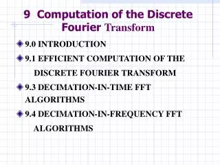
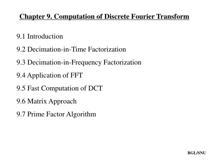
Chapter 9. Computation of Discrete Fourier Transform. 9.1 Introduction 9.2 Decimation-in-Time Factorization 9.3 Decimation-in-Frequency Factorization 9.4 Application of FFT 9.5 Fast Computation of DCT 9.6 Matrix Approach 9.7 Prime Factor Algorithm. BGL/SNU. 1. Introduction. BGL/SNU.

E N D
Chapter 9. Computation of Discrete Fourier Transform 9.1 Introduction 9.2 Decimation-in-Time Factorization 9.3 Decimation-in-Frequency Factorization 9.4 Application of FFT 9.5 Fast Computation of DCT 9.6 Matrix Approach 9.7 Prime Factor Algorithm BGL/SNU
1. Introduction BGL/SNU
- Example of fast computation BGL/SNU
3. Decimation-in-frequency Factorization (Sande- Tuckey) FFT BGL/SNU
g(n) h(n) g[0] g[1] g[2] g[3] h[0] h[1] h[2] h[3] x[0] x[1] x[2] x[3] x[4] x[5] x[6] x[7] X[0] X[2] X[4] X[6] X[1] X[3] X[5] X[7]
Final flow graph x[0] x[1] x[2] x[3] x[4] x[5] x[6] x[7] X[0] X[4] X[2] X[6] X[1] X[5] X[3] X[7] BGL/SNU
-Remarks • # Stages • # butterflies • # computations • inplace computations • output data ordering : bit-reversed • -Question • The flow graph for D-I-F is obtained by reversing. • The direction of the flow graph for D-I-T. Why? • -Omit Sections 9.5-9.7 BGL/SNU
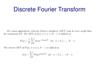
4. Applications of FFT (1) Spectrum Analysis - is the spectrum of x[n] , n=0,1,…,N-1 - Inverse transform can be done through the same mechanism i) Take the complex conjugate of X[k] ii) Pass it through the FFT process, But with one shift right(/2) operation at each stage iii) Finally, take the complex conjugate of the result BGL/SNU
h[n] 0 N-1 n y[n 0 2N-2 n - Operation reduction : (2) Convolution ( Filtering ) h[n] x[n] y[n] N 2N N x[n] 0 N-1 n #computation(multi)? 1+2+…+N+N-1+…+1+0 =N2
x[n] 0 N-1 2N n ~ h[n] 0 N-1 2N n R2N[n] 1 0 2N-1 n y[n] 0 2N-2 2N n ~ -Utilize FFT of 2N-point ~ 2N-pt DFTs BGL/SNU
X[k] 2N-pt FFT x[n] Y[k] 2N-pt IFFT y[n] 2N-pt FFT h[n] H[k] 2N • # operation (multi) • operation reduction : BGL/SNU
(3) Correlation /Power Spectrum 2N-point DFTs # Operation : • Power spectrum P[k] = X[k] X*[k] BGL/SNU
$ Comparison of # computation Direct Computation 106 1M 250k 105 FFT-based Convolution Correlation 62.5k 104 35k 16k 16k 7.25k FFT 103 3.3k 5k 2k 1k 102 0.45k 10 1 N 512 1024 BGL/SNU
5. Fast Computation of DCT BGL/SNU
- Example: Lee’s Algorithm (1984, IEEE Trans , ASSP, Dec) 1D X[0] X[4] X[2] X[6] X[1] X[5] X[3] X[7] x[0] x[1] x[2] x[3] x[4] x[5] x[6] x[7] BGL/SNU
- Example: 2D DCT Algorithm (1991, N.I.Cho and S.U.Lee) Separable Transform NxN 2D DCT = N 1-D DCT into row direction followed by N 1-D DCT into column direction. Totally 2N 1-D DCT (each N-point) are required. BGL/SNU
Fast Algorithm reduces the number of 1-D DCTs into N. By using the trigonometric properties, 2D DCT is decomposed into 1-D DCTs.
Signal flow graph of 2-D DCT 8x8 DCT 4x4 DCT
6. Matrix Approach · Decimation-in-time BGL/SNU
BGL/SNU
· Decimation-in-frequency BGL/SNU
· # computations (complex) BGL/SNU
7. Prime Factor Algorithm (Thomas/Good) (1) Basics from Number Theory Euler’s Phi function Euler’s Theorem N f = = ( ) If ( a , N ) 1 , then a 1 mod N . f = = f = = = ( N ) ( eg ) a 5 , N 6 , ( N ) 2 , a 25 1 mod 6 Chinese Remainder Theorem (CRT)
(2) Prime Factor Algorithm Set Then BGL/SNU
Therefore Note that the only difference is in the “twiddle factor” BGL/SNU
(3) Comparison Example 12-Point DFT (N=12, p=3, q=4) C/T : Cooley/Tuckey T/G : Thomas/Good · Transform · Index Mappings
4pt DFT 4pt DFT 3pt DFT 3pt DFT 3pt DFT 3pt DFT 4pt DFT x x ( ( k k , , n k ) ) 2 1 0 0 1 0 · Diagram X ( k , k ) 1 0 0 0 (0,0) 0 0 (0,0) (0,0) (1,0) 3 3 (0,1) (0,1) 4 4 6 6 (2,0) (0,2) (3,0) 9 9 (0,2) 8 8 (0,3) (1,0) 1 9 (1,1) 5 1 (1,0) 4 1 (0,1) (1,2) 9 5 (1,1) (1,1) 7 4 10 7 (2,1) (1,2) (2,0) 2 6 (3,1) 1 10 (1,3) (2,1) 6 10 (2,2) 10 2 (2,0) 8 2 (0,2) (3,0) 3 3 (1,2) (2,1) 11 5 (3,1) 7 7 2 8 (2,2) (2,2) (3,2) 5 11 (3,2) 11 (2,3) 11 C/T T/G C/T C/T T/G BGL/SNU
Radix-4 algorithm - Radix-2 algorithms: algorithms in textbook : - Radix-4 algorithms : BGL/JWL/SNU
- Radix-4 butterfly BGL/JWL/SNU
- Radix-4 butterfly -j -1 j -1 1 -1 j -1 -j BGL/JWL/SNU